Seasonality (Supply Chain)

In supply chain, the demand - or the sales - of a given product is said to exhibit seasonality when the underlying time-series undergoes a predictable cyclic variation depending on the time within the year. Seasonality is one of most frequently used statistical patterns to improve the accuracy of demand forecasts.

Illustration of seasonal time-series

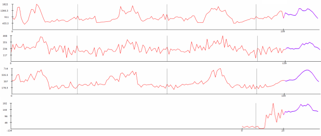
The graph below illustrates 4 seasonal time-series (click to enlarge). Time-series are aggregated at the weekly level over a period of 159 weeks (roughly 3 years). The data represent weekly shipments for 4 distinct products from the warehouse of a large European retailer.

The first day of the year (January 1st) is marked with a gray vertical marker. The historical data appears in red while the Lokad forecast is displayed in purple. The seasonality can be visually observed as a similarity of the patterns from one year to the next; use the gray markers as references.

Basic model for seasonal decomposition

Let Y(t) be the demand at the time t. We decompose the demand Y(t) into two components: S(t) a strictly cyclical function and Z(t) the non-seasonal complement. This gives:

Y(t) = S(t) * Z(t) where S(t + 1 year) = S(t)

If such a function S(t) can be estimated, then the forecasting process typically goes in three stages:

• Compute the deseasonalized time-series as Z(t) = Y(t) / S(t).
• Produce the forecast over the time-series Z(t), possibly through moving average.
• Re-apply the seasonality indices to the forecast afterward.

Back to the initial problem of estimating the seasonal indices S(t), assuming there is no trend (among other), S(t) can be estimated with:

S(t) = AVERAGE( Y(t-1)/MA(t-1) + Y(t-2)/MA(t-2) + Y(t-3)/MA(t-3) + ... )

where Y(t-1) is the shortcut for Y(t - 1 year) and MA(t) the 1-year moving average of Y(t).

The approach propose in this section is naive, but can be easily implemented in Excel. Many statistical models can be found in the literature to tackle seasonality with more complicated methods. Ex: Box-Jenkins, ARMA, ARIMA, Holt-Winters…

Challenges in estimating seasonality indices

The seasonality model illustrated here above is a rather naive approach that work for long smooth seasonal time-series. Yet, there are multiple practical difficulties when estimating seasonality:

1. Time-series are short. The lifespan of most consumer goods do not exceed 3 or 4 years. As a result, for a given product, sales history offers on average very few points in the past to estimate each seasonal index (that is to say the values of S(t) during the course of the year, cf. the previous section).
2. Time-series are noisy. Random market fluctuations impact the sales, and make the seasonality more difficult to isolate.
3. Multiple seasonalities are involved. When looking at sales at the store level, the seasonality of the product itself is typically entangled with the seasonality of the store.
4. Other patterns such as trend or product life-cycle also impact time-series, introducing various sort of bias in the estimation.

A simple - albeit manpower intensive - method to address those issues consists of manually creating seasonality profiles out of aggregates of products known to have the same seasonal behavior. The lifespan of the product aggregate is typically much longer than the lifespan of the individual products, which mitigates those estimation issues.

Quasi-seasonality

There are many patterns that happen once a year but not always at the same date. At Lokad, we call those patterns quasi-seasonal. For example, Mother’s Day (which falls on different dates depending on the year and also varies between countries) and other holidays like Ramadan, Easter and Hanukkah (which fall on different dates depending on the year), are quasi-seasonal.

Those quasi-seasonal events fall beyond the scope of classical cyclical forecasting models that assume that the period of the cycle is strictly constant. In order to deal with those quasi-seasonal events, a more complex quasi-cyclical logic is required.

Lokad’s gotcha

In our experience, seasonality impacts the vast majority of human activities. In particular, in time-series representing sales of consumer goods (food and non-food alike), a seasonal factor is nearly always present. However, it frequently happens that, due to the amount of market noise, the quality of the estimation of the seasonal indices ends up too low to be practical use to refine the forecasts.

The forecasting technology of Lokad natively handles both seasonality and quasi-seasonality, so you don’t have to tell Lokad about them, it’s already taken care of.

In order to overcome issues raised by the limited historical depth available for most time-series in retail or manufacturing, Lokad uses multiple time-series analysis and the seasonality is evaluated not on a single product but looking at many products. By doing this, we reduce the noise in our estimation of the seasonality, but also introduce seasonality in the forecasts even when products have been sold for less than a year.