00:17 Introduction
03:35 Orders of Magnitude
06:55 Stages of Supply Chain Optimization
12:17 The S-Curves of hardware
15:52 The story so far
17:34 Auxiliary sciences
20:25 Modern computers
20:57 Latency 1/2
27:15 Latency 2/2
30:37 Compute, clock speed
36:36 Compute, pipelining, 1/3
39:11 Compute, pipelining, 2/3
40:27 Compute, pipelining, 3/3
46:36 Compute, superscalar 1/2
49:55 Compute, superscalar 2/2
56:45 Memory 1/3
01:00:42 Memory 2/3
01:06:43 Memory 3/3
01:11:13 Data storage 1/2
01:14:06 Data storage 2/2
01:18:36 Bandwidth
01:23:20 Conclusion
01:27:33 Upcoming lecture and audience questions
Description
Modern supply chains require computing resources to operate just like motorized conveyor belts require electricity. Yet, sluggish supply chain systems remain ubiquitous, while the processing power of computers has increased by a factor greater than 10,000x since 1990. A lack of understanding of the fundamental characteristics of modern computing resources - even among IT or data science circles - goes a long way in explaining this state of affairs. The software design underlying the numerical recipes shouldn’t antagonize the underlying computing substrate.
Full transcript
Welcome to this series of supply chain lectures. I’m Joannes Vermorel, and today I will be “Presenting Modern Computers for Supply Chain.” Western supply chains have been digitalized for a long time, sometimes up to three decades ago. Computer-based decisions are everywhere, and the associated numerical recipes go under various names such as reorder points, min-max inventory, and safety stocks, with varying degrees of human supervision.
Nonetheless, if we look at large companies nowadays who operate equivalently large supply chains, we see millions of decisions that are essentially computer-driven, which drive the performance of the supply chain. Thus, when it comes to the improvement of the supply chain performance, it quickly boils down to the improvement of the numerical recipes that drive the supply chain. Here, invariably, when we start considering superior numerical recipes of any kind, where we want better models and more accurate forecasts, those superior recipes end up costing a lot more computing resources.
Computing resources have been a struggle for supply chain as they cost a lot of money, and there is always the next stage of evolution for the next model or the next forecasting system that requires ten times more computing resources than the previous one. Yes, it could bring extra supply chain performance, but it comes with increased computing cost. Over the last couple of decades, computing hardware has been progressing tremendously, but as we will see today, this progress, although still ongoing, is frequently antagonized by enterprise software. As a result, software doesn’t get faster with more modern hardware; on the contrary, it can very frequently get slower.
The goal for this lecture is to instill among the audience some degree of mechanical sympathy, so you can assess whether a piece of enterprise software that is supposed to implement numerical recipes intended to deliver superior supply chain performance embraces the computing hardware as it already exists and as it will exist a decade from now, or does it antagonize and thus essentially not make the most of the computing hardware that we have today.
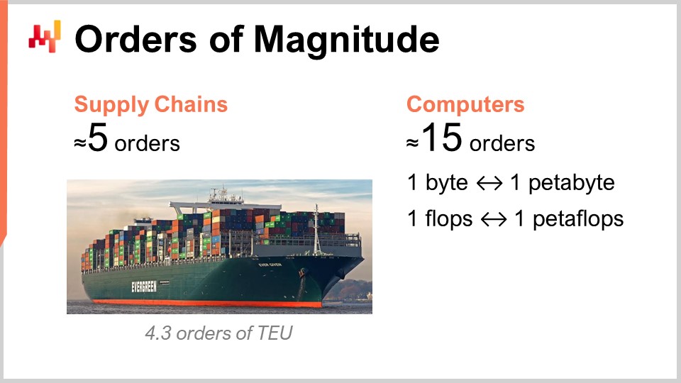
One of the most puzzling aspects of modern computers is the range of orders of magnitude that are involved. From the supply chain perspective, we typically have about five orders of magnitude, and that’s already stretching it; usually, it’s not even that. Five orders of magnitude means that we can go from one unit to 100,000 units. Remember that something I discussed in previous lectures is the law of small numbers at play. If you have a large number of units, you’re not going to process those units individually; you’re going to pack them into boxes, and thus you will be left with a much smaller number of boxes. Similarly, if you have many boxes, you will pack them into pallets, etc., so that you have a much smaller number of pallets. Economies of scale induce predictions of quantities, and from the supply chain perspective, when we are dealing with the flow of physical goods, a 10% inefficiency tends to be already quite significant.
In the realm of computers, it’s very different; we are dealing with 15 orders of magnitude, which is absolutely gigantic. To go from one unit to one million billion units, the number is so large that it’s actually very difficult to visualize. We go from one byte, which is just eight bits and can be used to represent a letter or a digit, to a petabyte, which is a million gigabytes. A petabyte is about the order of magnitude of the amount of data that Lokad presently manages, and large companies operating large supply chains are also operating datasets of the order of magnitude of one petabyte.
We go from one FLOP (floating point operation per second) to one petaFLOP, which is one million gigaFLOPS. These orders of magnitude are absolutely gigantic and very deceptive. As a result, in the supply chain realm, where 10% is considered inefficient, what typically happens in the realm of computers is that it’s not about being inefficient by 10%, it’s more about being inefficient by a factor of 10, and sometimes several orders of magnitude. So, if you do something wrong in terms of performance in the realm of computers, your penalty will not be 10%; instead, your system is going to be 10 times slower than it should be, or 100 times, and sometimes even a thousand times slower than it should have been. That’s really what’s at stake: having a true alignment, which requires some kind of mechanical sympathy between the enterprise software and the underlying computing hardware.
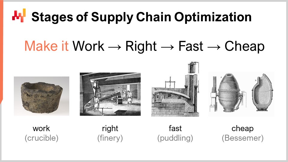
When considering a numerical recipe that is supposed to deliver some kind of superior supply chain performance, there is a set of stages of maturity that are of interest conceptually. Obviously, your mileage may vary in practice, but that’s typically what we have identified at Lokad. These stages can be summarized as: make it work, make it right, make it fast, and make it cheap.
“Make it work” is about assessing whether a prototype numerical recipe is really delivering the intended results, such as higher service levels, less dead stock, better utilization of assets, or any other goal that is worthy from a supply chain perspective. The goal is first to make sure that the new numerical recipe actually works at the first stage of maturity.
Then, you have to “make it right.” From a supply chain perspective, this means transforming what was essentially a unique prototype into something with production-grade quality. This typically involves attaching to the numerical recipe some degree of correctness by design. Supply chains are vast, complex, and, more importantly, very messy. If you have a numerical recipe that is very fragile, even if the numerical method is good, it’s very easy to get it wrong, and then you end up creating many times more problems compared to the benefits you intended to bring in the first place. This is not a winning proposition. Making it right is to ensure that you have something that can be deployed at scale with minimal friction. Then, you want to make this numerical recipe fast, and when I say fast, I mean fast in terms of wall clock time. When you start the calculation, you should get the results within minutes, or maybe an hour or two at most, but no longer. Supply chains are messy, and there will be a point in time in the history of your company where there will be disruptions, such as container ships stuck in the middle of the Suez Canal, a pandemic, or a warehouse getting flooded. When this happens, you need to be able to react quickly. I’m not saying react in the next milliseconds, but if you have numerical recipes that take days to complete, it creates massive operational friction. You need things that can be operated within a short human timeframe, so it needs to be fast.
Remember, modern enterprise software runs on clouds, and you can always pay for more computing resources on cloud computing platforms. Thus, your software can actually be fast just because you are renting lots of processing power. It’s not that the software itself has to be properly designed to leverage all the processing power that a cloud can provide, but it can be fast and very inefficient just because you’re renting so much processing power from your cloud computing provider.
The next stage is to make the method cheap, meaning that it doesn’t use too many cloud computing resources. If you don’t go into this final stage, it means that you can never improve upon your method. If you have a method that works, is right, and is fast but consumes a lot of resources, when you want to move on to the next stage of numerical recipe, which will invariably involve something that costs even more computing resources than what you’re currently using, you’ll be stuck. You need to make the method you have super lean so that you can start experimenting with numerical recipes that are less efficient than what you currently have.
This last stage is where you really need to embrace the underlying hardware that is available in modern computers. You can manage with the first three stages without too much affinity, but the last one is key. Remember, if you don’t get to the “make it cheap” stage, you won’t be able to iterate, and so you’ll be stuck. That’s why, even if it’s the last stage, this is an iterative game, and it’s essential to go through all the stages if you want to repeatedly iterate.
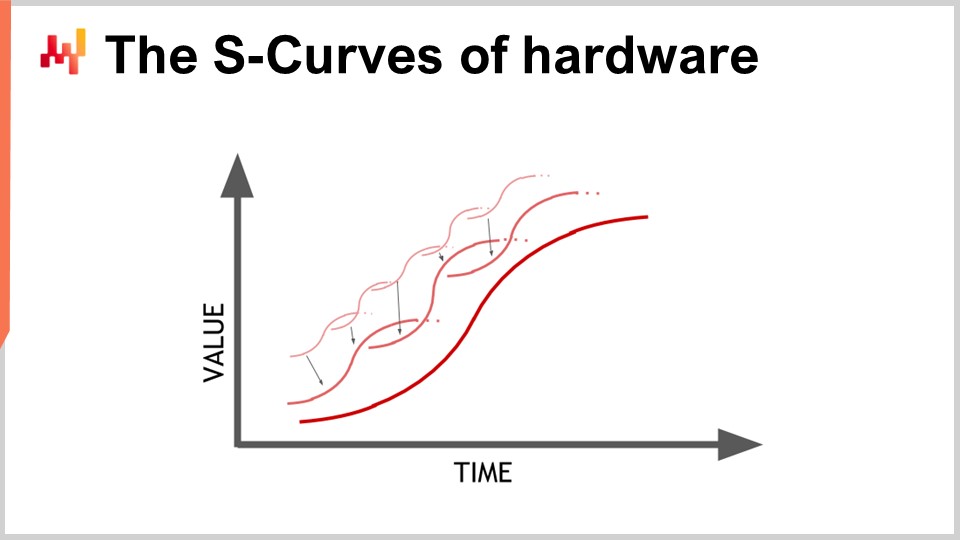
Hardware is progressing, and it looks like an exponential progression, but the reality is that this exponential progression of computing hardware is actually made up of thousands of S-curves. An S-curve is a curve where you introduce a new design, process, material, or architecture, and initially, it’s not really better than what you had before. Then, the effect of the intended innovation kicks in, and you have a ramp-up, followed by a plateau after you consume all the benefits of the innovation. Plateauing S-curves are characteristic of the progress in computer hardware, which is made up of thousands of these curves. From a layman’s perspective, this appears as exponential growth. However, experts see the individual S-curves plateauing, which can lead to a pessimistic view. Even the experts don’t always see the emergence of new S-curves that surprise everyone and continue the exponential growth of progress.
Although computing hardware is still progressing, the rate of progress is nowhere near what we experienced in the 1980s or 1990s. The pace is now much slower and quite predictable, largely due to the massive investments required to build new factories for producing computing hardware. These investments often amount to hundreds of millions of dollars, providing visibility five to ten years ahead. While progress has slowed down, we still have a fairly accurate view of what will happen in terms of computing hardware progress for the next decade.
The lesson for enterprise software implementing numerical recipes is that you cannot passively expect future hardware to make everything better for you. Hardware is still progressing, but capturing this progress requires effort from the software side. You will be able to do more with the hardware that exists a decade from now, but only if the architecture at the core of your enterprise software embraces the underlying computing hardware. Otherwise, you might actually do worse than what you’re doing today, a proposition that is not as unreasonable as it sounds.
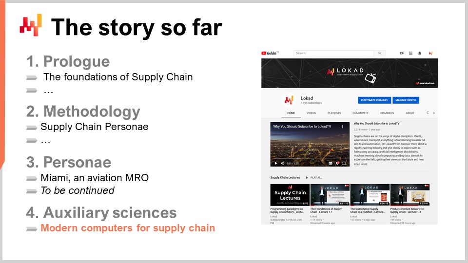
This lecture is the first of the fourth chapter in this series of supply chain lectures. I have not finished the third chapter about supply chain personae. In the following lectures, I will likely alternate between the present chapter, where I’m covering the auxiliary sciences of supply chain, and the third chapter on supply chain personae.
In the very first chapter of the prologue, I presented my views on supply chain as both a field of study and a practice. We have seen that supply chain is essentially a collection of wicked problems, as opposed to tame problems, plagued by adversarial behavior and competitive games. Therefore, we need to pay a great deal of attention to methodology because naive direct methodologies perform poorly in this field. That’s why the second chapter was dedicated to the methodology needed to study supply chains and establish practices to improve them over time.
The third chapter, Supply Chain Personae, focused on characterizing the supply chain problems themselves, with the motto “fall in love with the problem, not with the solution.” The fourth chapter that we are opening today is about the auxiliary sciences of supply chains.
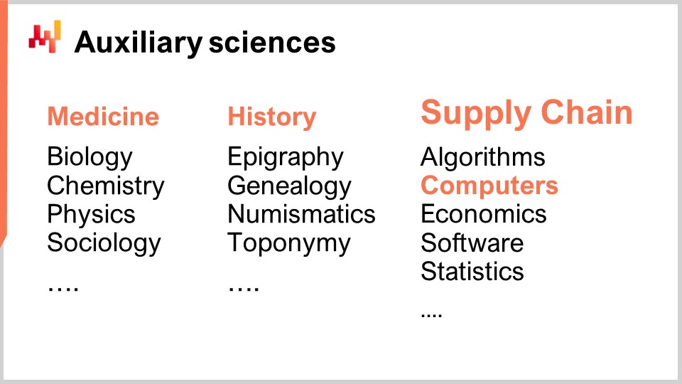
Auxiliary sciences are disciplines that support the study of another discipline. There is no judgment of value; it’s not about one discipline being superior to another. For example, medicine is not superior to biology, but biology is an auxiliary science for medicine. The perspective of auxiliary sciences is well-established and prevalent in many fields of research, such as medical sciences and history.
In medical sciences, auxiliary sciences include biology, chemistry, physics, and sociology, among others. A modern physician would not be considered competent if they had no knowledge of physics. For instance, understanding the basics of physics is necessary to interpret an X-ray image. The same is true for history, which has a long series of auxiliary sciences.
When it comes to supply chain, one of my biggest criticisms of typical supply chain materials, courses, books, and papers is that they treat the subject without delving into any auxiliary sciences. They treat supply chain as if it were an isolated, self-standing piece of knowledge. However, I believe that modern supply chain practice can only be achieved by fully leveraging the auxiliary sciences of supply chains. One of these auxiliary sciences, and the focus of today’s lecture, is computing hardware.
This lecture is not strictly a supply chain lecture, but rather computing hardware with supply chain applications in mind. I believe it is fundamental for practicing supply chain in a modern way, as opposed to how it was done a century ago.
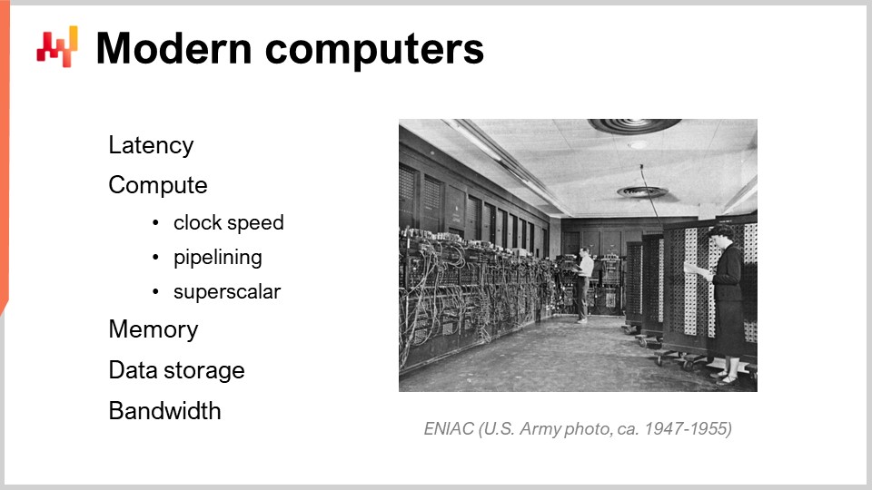
Let’s have a look at modern computers. In this lecture, we will review what they can do for supply chain, particularly focusing on aspects that have a massive impact on the performance of enterprise software. We will review latency, compute, memory, data storage, and bandwidth.

The speed of light is about 30 centimeters per nanosecond, which is relatively slow. If you consider the characteristic distance of interest for a modern CPU that operates at 5 gigahertz (5 billion operations per second), the round trip distance that light can travel in 0.2 nanoseconds is only 3 centimeters. This means that, due to the limitation of the speed of light, interactions cannot occur beyond 3 centimeters. This is a hard limitation imposed by the laws of physics, and it’s unclear whether we will ever be able to overcome it.
Latency is an exceedingly hard constraint. From a supply chain perspective, we have at least two distributions of computing hardware involved. When I say distributed computing hardware, I mean computing hardware that involves many devices that cannot occupy the same physical space. Obviously, you need to keep them apart just because they have dimensions of their own. However, the first reason we need distributed computing is the nature of supply chains, which are geographically distributed. By design, supply chains are spread across geographies, and thus, there will be computing hardware spread over those geographies as well. From the speed of light perspective, even if you have devices that are only three meters apart, it’s already very slow because it takes 100 clock cycles to do the round trip. Three meters is quite a distance from the perspective of the speed of light and the clock rate of modern CPUs.
Another type of distribution is horizontal scaling. The modern way of having more processing power at our disposal is not to have a computing device that is 10 times or a million times more powerful; that’s not how it is engineered. If you want more processing resources, you need extra computing devices, more processors, more memory chips, and more hard drives. It’s by piling up the hardware that you can have more computational resources at your disposal. However, all those devices take space, and thus, you end up distributing your computing hardware just because you can’t centralize it into a centimeter-wide computer.
When it comes to latencies, looking at the sort of latencies we have on the professional internet (the latencies you can get in a data center, not over your Wi-Fi at home), we are already within 30% of the speed of light. For example, the latency between a data center near Paris, France, and New York, United States, is only within 30% of the speed of light. This is an incredible achievement for mankind; information is flowing across the internet at near the speed of light. Yes, there is still room for improvement, but we are already close to the hard limits imposed by physics.
As a result, there are even companies now that want to lay cable through the Arctic sea floor to connect London to Tokyo with a cable that would go under the North Pole, just to shave a few milliseconds of latency for financial transactions. Fundamentally, latency and the speed of light are very real concerns, and the internet we have is essentially as good as it will ever be unless there are breakthroughs in physics. However, we have nothing like that looming ahead for the next decade.
Due to the fact that latency is a super hard problem, the implications for enterprise software are significant. Round trips in terms of the flow of information are deadly, and the performance of your enterprise software will largely be dependent on the number of round trips between the various subsystems that exist within your software. The number of round trips will characterize the incompressible latency that you suffer. Minimizing round trips and improving latencies is, for most pieces of enterprise software, including those dedicated to the predictive optimization of supply chains, the number one problem. Mitigating latencies often equates to delivering better performance.
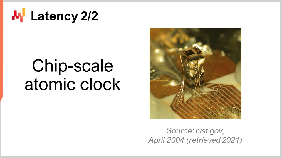
An interesting trick, although not something that everyone in this audience will deploy in production, is addressing the complications introduced by latency. Time itself becomes elusive and fuzzy when you enter the realm of nanosecond calculations. Accurate clocks are hard to come by in distributed computing, and their absence introduces complications within distributed enterprise software. Numerous round trips are needed to synchronize the various pieces of the system. Due to the lack of an accurate clock, you end up with algorithmic alternatives such as vector clocks or multi-part timestamps, which are data structures that reflect a partial ordering of device clocks in your system. These extra round trips can hurt performance.
A clever design adapted by Google over a decade ago was to use chip-scale atomic clocks. The resolution of these atomic clocks is significantly better than that of quartz-based clocks found in electronic watches or computers. NIST demonstrated a new setup of chip-scale atomic clock with an even more precise daily drift. Google used internal atomic clocks to synchronize the various parts of their globally distributed SQL database, Google Spanner, to save round trips and improve performance at a global scale. This is a way to cheat latency through very precise time measurements.
Looking a decade ahead, Google will likely not be the last company to use this sort of clever trick, and they are relatively affordable, with chip-scale atomic clocks costing around $1,500 a piece.
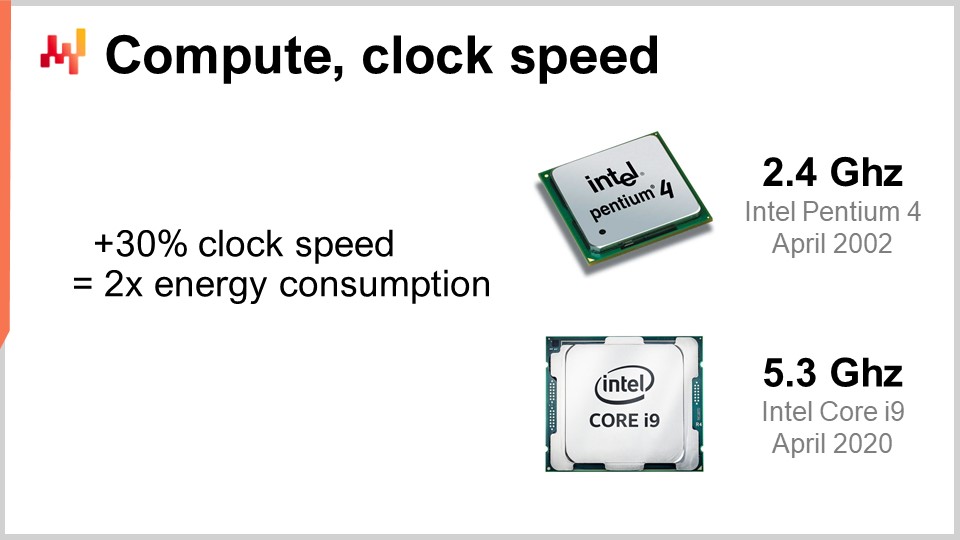
Now, let’s have a look at compute, which is about doing computations with a computer. The clock speed was the magical ingredient of improvement during the 80s and 90s. Indeed, if you could double the clock speed of your computer across the board, you would effectively double the performance of your computer, no matter which kind of software is involved. All software would be linearly faster according to the clock speed. It is extremely interesting to increase the clock speed, and it is still improving, although the improvement has flattened over time. Almost 20 years ago, the clock speed was about 2 GHz, and nowadays, it is 5 GHz.
The key reason for this flattened improvement is the power wall. The problem is that when you increase the clock speed on a chip, you tend to roughly double the energy consumption, and then you have to dissipate this energy. The issue is thermal dissipation because, if you can’t dissipate the energy, your device builds up heat to the point where it damages the device itself. Nowadays, the semiconductor industry has moved from having more operations per second to more operations per watt.
This rule of a 30% increase doubling the energy consumption is a double-edged sword. If you are okay with giving up a quarter of your processing power per unit of time on the CPU, you can actually divide the power consumption by two. This is especially interesting for smartphones, where energy savings are crucial, and also for cloud computing, where one of the key drivers of cost is the energy itself. To have cost-effective cloud computing processing power, it is not about having super-fast CPUs, but rather about having underclocked CPUs that can be as slow as 1 GHz, as they provide more operations per second for your energy investment.
The power wall is such a problem that modern CPU architectures are using all sorts of clever tricks to mitigate it. For example, modern CPUs can regulate their clock speed, temporarily boosting it for a second or so before reducing it to dissipate heat. They can also leverage what is called dark silicon. The idea is that if the CPU can alternate the hot areas on the chip, it is easier to dissipate the energy as opposed to always having the same area active clock cycle after clock cycle. This is a very key ingredient of modern design. From an enterprise software perspective, it means that you really want to be able to scale out. You want to be able to do more with many times more CPUs, but individually, those processors are going to be weaker than the previous ones you had. It’s not about getting better processors in the sense that everything is better across the board; it’s about having processors that give you more operations per watt, and this trend will continue.
Maybe a decade from now, we will reach, with difficulty, seven or maybe eight gigahertz, but I’m not even sure that we will get there. When I look at the clock speed in 2021 in most cloud computing providers, it’s more aligned with typically 2 GHz, so we are back to the clock speed we had 20 years ago, and that is the most cost-effective solution.
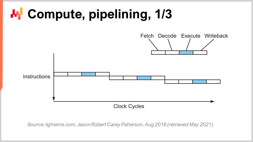
Reaching the present CPU performance required a series of key innovations. I’m going to present a few of them, especially the ones that have the most impact on the design of enterprise software. On this screen, what you’re seeing is the instruction flow of a sequential processor, as processors were made essentially up to the early 80s. You have a series of instructions that execute from the top of the graph to the bottom, representing time. Every instruction goes through a series of stages: fetch, decode, execute, and write back.
During the fetch stage, you fetch the instruction, register, grab the next instruction, increment the instruction counter, and prepare the CPU. During the decode stage, you decode the instruction and emit the internal microcode, which is what the CPU is executing internally. The execution stage involves grabbing the relevant inputs from the registers and doing the actual calculation, and the write back stage involves getting the result you’ve just computed and putting it somewhere in one of the registers. In this sequential processor, every single stage requires one clock cycle, so it takes four clock cycles to execute one instruction. As we have seen, it is very difficult to increase the frequency of the clock cycles themselves because of many complications.
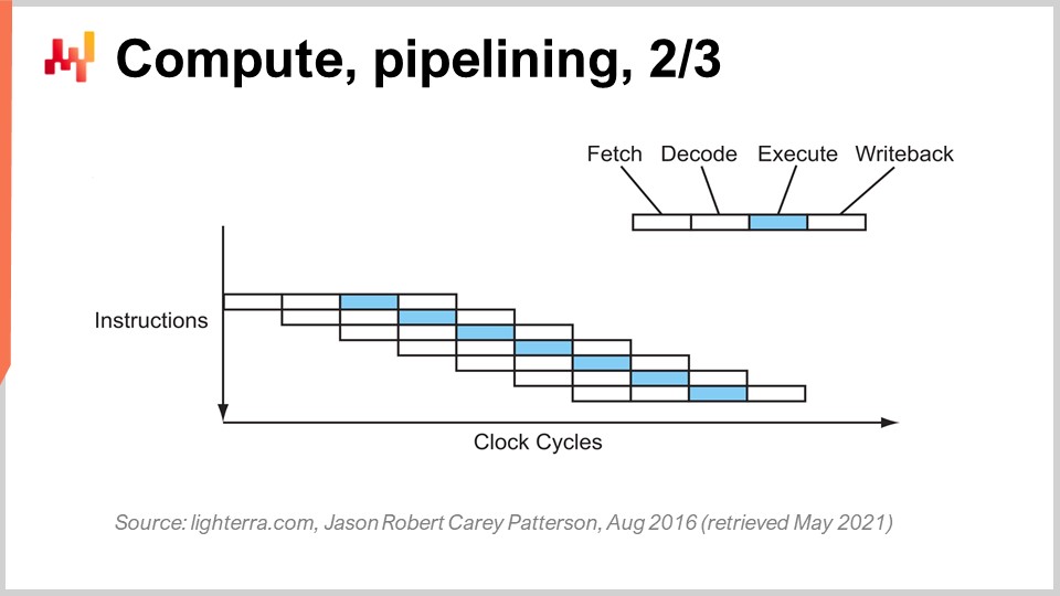
The key trick that has been in place since the early 80s and onward is known as pipelining. Pipelining can enormously speed up the calculation of your processor. The idea is that, due to the fact that every single instruction goes through a series of stages, we are going to overlap the stages, and thus the CPU itself is going to have a whole pipeline of instructions. On this diagram, you can see a CPU with a pipeline of depth four, where there are always four instructions being executed concurrently. However, they are not in the same stage: one instruction is in the fetch stage, one in the decode stage, one in the execute stage, and one in the write-back stage. With this simple trick, represented here as a pipeline processor, we have multiplied the effective performance of the processor by four by just pipelining the operations. All modern CPUs use pipelining.
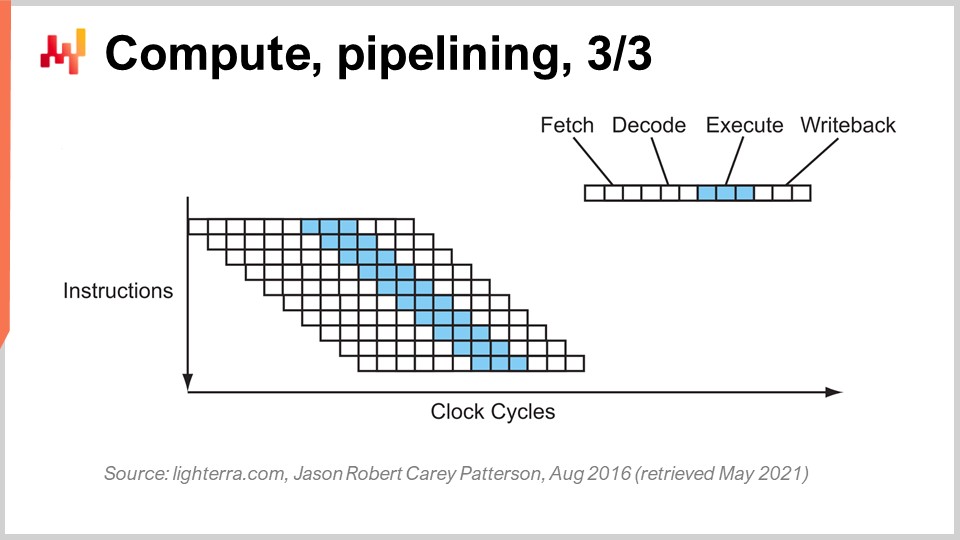
The next stage of this improvement is called super pipelining. Modern CPUs go way beyond simple pipelining. In reality, the number of stages involved in a real modern CPU is more like 30 stages. On the graph, you can see a CPU with 12 stages as an example, but in reality, it would be more like 30 stages. With this deeper pipeline, 12 operations can execute concurrently, which is very good for performance while still using the same clock cycle.
However, there’s a new problem: the next instruction starts before the previous one is finished. This means that if you have operations that are dependent, you have a problem because the calculation of the inputs for the next instruction is not ready yet, and you have to wait. We want to utilize the entire pipeline at our disposal to maximize processing power. Thus, modern CPUs fetch not just one instruction at a time, but something like 500 instructions at a time. They look far ahead in the list of upcoming instructions and rearrange them to mitigate dependencies, interleaving the execution flows to leverage the full depth of the pipeline.
There are plenty of things that complicate this operation, most notably branches. A branch is just a condition in programming, such as when you write an “if” statement. The result of the condition can be true or false, and depending on the result, your program will execute one piece of logic or another. This complicates the dependency management because the CPU has to guess the direction the upcoming branches are going to go. Modern CPUs use branch prediction, which involves simple heuristics and has very high forecasting accuracy. They can predict the direction of branches with over 99% accuracy, which is better than what most of us can do in a real supply chain context. This precision is needed to leverage super deep pipelines.
Just to give you an idea of the sort of heuristics used for branch prediction, a very simple heuristic is to say the branch will go the same way, in the same direction, it went last time. This simple heuristic gives you something like 90% accuracy, which is quite good. If you add a twist to this heuristic, which is that the branch will go in the same direction as last time, but you need to consider the origin, so it’s the same branch coming from the same origin, then you will get something like 95% accuracy. Modern CPUs are actually using fairly complex perceptrons, which is a machine learning technique, to predict the direction of the branches.
Under the right conditions, you can predict branches fairly accurately and thus leverage the full pipeline to get the most out of a modern processor. However, from a software engineering perspective, you need to play nice with your processor, especially with branch prediction. If you don’t play nice, it means that the branch predictor will get it wrong, and when that happens, the CPU will predict the direction of the branch, organize the pipeline, and start doing calculations ahead of time. When the branch is actually encountered and the calculation is effectively done, the CPU will realize that the branch prediction was wrong. An incorrect branch prediction does not result in an incorrect result; it results in a loss of performance. The CPU will have no alternative but to flush the entire pipeline, or a large portion of it, wait until other calculations are made, and then restart the calculation. The performance hit can be very significant, and you can very easily lose one or two orders of magnitude in performance due to enterprise software logic that does not play well with the branch prediction logic of your CPU.
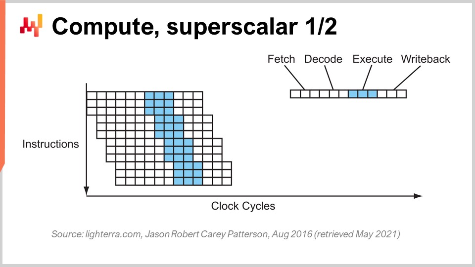
Another notable trick beyond pipelining is superscalar instruction. CPUs typically process scalars, or pairs of scalars, at a time – for example, two numbers with 32-bit floating-point precision. They perform scalar operations, essentially processing one number at a time. However, modern CPUs for the last decade have pretty much all featured superscalar instruction, which can actually process several vectors of numbers and perform vector operations directly. This means that a CPU can take a vector of, let’s say, eight floating-point numbers and a second vector of eight floating-point numbers, perform an addition, and get a vector of floating-point numbers that represent the results of this addition. All of that is done in one cycle.
For example, specialized instruction sets like AVX2 let you perform operations considering 32 bits of precision with packs of eight numbers, while AVX512 lets you do that with packs of 16 numbers. If you’re capable of leveraging these instructions, it means that you can literally gain an order of magnitude in terms of processing speed because one instruction, one clock cycle, does many more calculations than processing numbers one by one. This process is known as SIMD (Single Instruction, Multiple Data), and it is very powerful. It has been driving the bulk of progress over the last decade in terms of processing power, and modern processors are increasingly vector-based and superscalar. However, from an enterprise software perspective, it is relatively tricky. With pipelining, your software has to play nice, and maybe it’s playing nice with the branch prediction accidentally. However, when it comes to superscalar instruction, there is nothing accidental. Your software really needs to do some things explicitly, most of the time, to leverage this extra processing power. You don’t get it for free; you need to embrace this approach, and typically, you need to organize the data itself so that you have data parallelism, and the data is organized in a way that is suitable for SIMD instructions. It’s not rocket science, but it doesn’t happen accidentally, and it gives you a massive boost in terms of processing power.
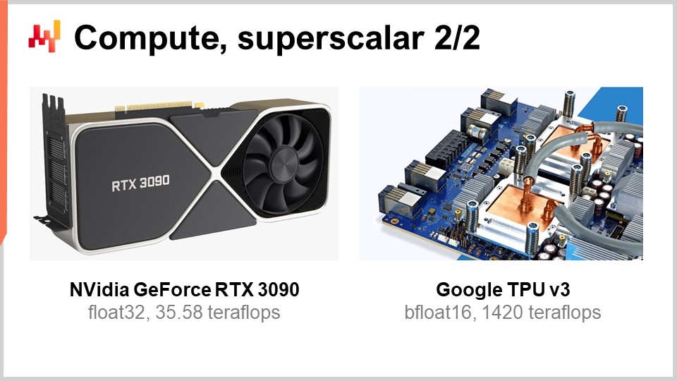
Now, modern CPUs can have many cores, and one CPU core can give you a distinct flow of instructions. With very modern CPUs that have many cores, typically, present-day CPUs can go up to 64 cores, so 64 independent concurrent flows of execution. You can pretty much reach about one teraflop, which is the upper limit of processing throughput that you can get from a very modern processor. However, if you want to go beyond that, you can look at GPUs (Graphical Processing Units). Despite what you might think, these devices can be used for tasks that have nothing to do with graphics.
A GPU, like the one from NVIDIA, is a superscalar processor. Instead of having up to 64 cores like high-end CPUs, GPUs can have more than 10,000 cores. These cores are much simpler and not as powerful or fast as regular CPU cores, but there are many times more of them. They bring SIMD to a new level, where you can crunch not only packs of 8 or 16 numbers at a time but literally thousands of numbers at a time to perform vector instructions. With GPUs, you can achieve a range of 30-plus teraflops on just one device, which is enormous. The best CPUs on the market may give you one teraflop, while the best GPUs will give you 30-plus teraflops. That’s more than an order of magnitude of difference, which is very significant.
If you go even beyond that, for specialized types of calculations such as linear algebra (by the way, things like machine learning and deep learning are essentially matrix-involved linear algebra all over the place), you can have processors like TPUs (Tensor Processing Units). Google decided to name them Tensors because of TensorFlow, but the reality is that TPUs would be better named Matrix Multiplication Processing Units. The interesting thing with matrix multiplication is that not only is there a ton of data parallelism involved, but there is also an enormous amount of repetition involved because the operations are highly repetitive. By organizing a TPU as a systolic array, which is essentially a two-dimensional grid with computational units on the grid, you can breach the petaflop barrier – achieving 1000-plus teraflops on just a single device. However, there is a caveat: Google is doing it with 16-bit floating point numbers instead of the usual 32-bit. From a supply chain perspective, 16 bits of precision is not bad; it means you have about 0.1% accuracy in your operations, and for many machine learning or statistical operations, 0.1% accuracy is quite fine if done right and without accumulating bias.
What we see is that the path of progress in terms of computing hardware, when looking at just compute, has been to go for devices that are more specialized and more rigid. Thanks to this specialization, you can achieve enormous gains in processing power. If you go from superscalar instruction, you gain an order of magnitude; if you go for a graphics card, you gain one or two orders of magnitude; and if you go for pure linear algebra, you gain essentially two orders of magnitude. This is very significant.
By the way, all of these hardware designs are two-dimensional. Modern chips and processing structures are very flat. A modern CPU does not involve more than 20 layers, and since these layers are only a few microns thick, CPUs, GPUs, or TPUs are essentially flat structures. You might think, “What about the third dimension?” Well, it turns out that due to the power wall, which is the problem of dissipating energy, we can’t really go into the third dimension because we don’t know how to evacuate all the energy that is poured into the device.
What we can predict for the next decade is that these devices will remain essentially two-dimensional. From the enterprise software perspective, the biggest lesson is that you need to engineer data parallelism right at the core of your software. If you don’t do that, then you will not be able to capture all the progress that is happening as far as raw compute power is concerned. However, it cannot be an afterthought. It has to happen at the very core of the architecture, at the level at which you organize all the data that has to be processed in your systems. If you don’t do that, you will be stuck with the sort of processors we had two decades ago.
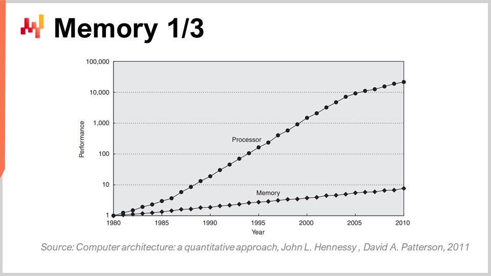
Now, memory in the early ’80s was as fast as processors, meaning that one clock cycle was one clock cycle for memory and one for the CPU. However, this is not the case anymore. Over time, since the ’80s, the ratio between the speed of memory and the latencies to access data already in the processor’s registers has only been increasing. We started with a ratio of one, and we now have a ratio typically greater than a thousand. This problem is known as the memory wall, and it has only been increasing over the last four decades. It is still increasing nowadays, although very slowly, primarily because the clock speed of processors is increasing very slowly. Due to the fact that processors are not progressing much in terms of clock speed, this problem of the memory wall is not increasing any further. However, the place we are left at the moment is incredibly imbalanced, where accessing memory is essentially three orders of magnitude slower than accessing data that already sits conveniently inside the processor.
This perspective completely defeats all the classic algorithmics as they are still taught nowadays in most universities. The classic algorithmic viewpoint assumes that you have a uniform time to access memory, meaning that accessing any bit of memory takes the same amount of time. But in modern systems, this is absolutely not the case. The time it takes to access a certain portion of memory very much depends on where the actual data is physically within your computer system.
From an enterprise software perspective, it turns out that unfortunately, most of the software designs that were established during the ’80s and ’90s ignored the problem altogether because it was very minor during the first decade. It only really inflated over the last two decades, but as a result, most of the patterns seen in present-day pieces of enterprise software completely antagonize this design, because they assume that you have constant time access for all memory.
By the way, if you start thinking about programming languages like Python (first released in 1989) or Java (in 1995) featuring object-oriented programming, it goes very much against the way memory works in modern computers. Whenever you have objects, and it’s even worse if you have late bindings like in Python, it means that to do anything, you will have to follow pointers and do random jumps into memory. If one of those jumps happens to be unlucky because it’s a portion that is not already sitting in the processor, it can be a thousand times slower. That’s a very big problem.
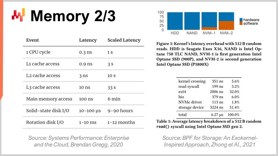
To better grasp the extent of the memory wall, it’s interesting to look at the typical latencies in a modern computer. If we rescale those latencies in human terms, let’s assume a processor was operating at one clock cycle per second. Under that assumption, the typical latency of the CPU would be one second. However, if we want to access data in memory, it could take up to six minutes. So, while you can perform one operation per second, if you want to access something in memory, you have to wait six minutes. And if you want to access something on disk, it can take up to a month or even a whole year. This is incredibly long, and that’s what those orders of magnitude of performance that I mentioned at the very beginning of this lecture are about. When you’re dealing with 15 orders of magnitude, it is very deceptive; you don’t necessarily realize the massive performance hit that you can have, where literally you can end up having to wait the human equivalent of months if you’re not putting the information in the right place. This is absolutely gigantic.
By the way, enterprise software engineers are not the only ones struggling with this evolution of modern computing hardware. If we look at the latencies that we get with super-fast SSD cards, such as the Intel Optane series, you can see that half of the latency to access the memory on this device is actually caused by the overhead of the kernel itself, in this case, the Linux kernel. It’s the operating system itself that generates half of the latency. What does that mean? Well, it means that even the people who are engineering Linux have some further work to do to catch up with modern hardware. Nonetheless, it’s a big challenge for everybody.
However, it really hurts enterprise software, especially when thinking about supply chain optimization, due to the fact that we have tons of data to process. It’s already quite a complex undertaking from the start. From the enterprise software perspective, you really need to embrace a design that plays nicely with the cache because the cache contains local copies that are faster to access and closer to the CPU.
The way it works is that when you access a byte in your main memory, you can’t access just one byte in modern software. When you want to access even one byte in your RAM, the hardware will actually copy 4 kilobytes, essentially the whole page that is 4 kilobytes large. The underlying assumption is that when you start to read a byte, the next byte that you’re going to request is going to be the one that follows. That’s the locality principle, which means that if you play by the rule and enforce access that preserves locality, then you can have memory that appears to work almost as fast as your processor.
However, that requires alignment between memory accesses and the locality of the data. In particular, there are plenty of programming languages, like Python, that do not deliver these sorts of things natively. On the contrary, they present a massive challenge to bring any degree of locality. This is an immense struggle, and ultimately, it’s a battle where you have a programming language that has been designed around patterns that completely antagonize the hardware at our disposal. This problem is not going to change in the coming decade; it’s only going to get worse.
Thus, from an enterprise software perspective, you want to enforce locality of the data but also minification. If you can make your big data small, it will be faster. That’s something that is not very intuitive, but if you can shrink the size of the data, typically by eliminating some redundancy, you can make your program faster because you will be much nicer with the cache. You will fit more relevant data in the lower cache levels that have much lower latencies, as shown on this display.
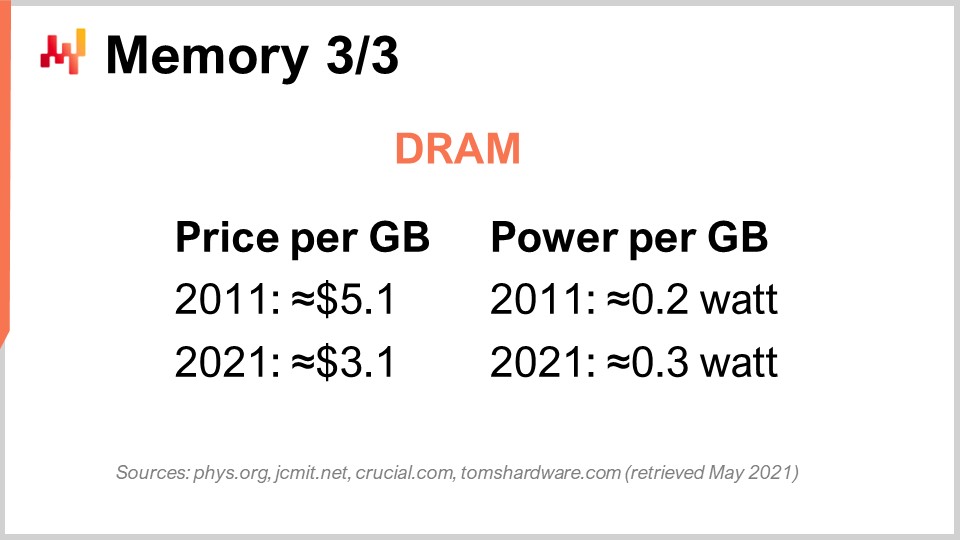
Finally, let’s discuss specifically the case of DRAM. DRAM is literally the physical component that builds up the RAM that you use for your desktop workstation or your server in the cloud. DRAM is also called the main memory, which is built from DRAM chips. Over the last decade, in terms of pricing, DRAM has barely decreased. We went from $5 per gigabyte to $3 per gigabyte a decade later. The price of RAM is still decreasing, although not very fast. It has been stagnating over the next couple of years, and due to the fact that there are only three major players in this market that have the capacity to manufacture DRAM at scale, there is very little hope that there will be anything unexpected in this market for the decade to come.
But that’s not even the worst of the problem. There is also the power consumption per gigabyte. If you look at the power consumption, it turns out that modern-day RAM is consuming a little bit more power per gigabyte than it used to one decade ago. The reason is essentially that the RAM we have presently is faster, and the same rule of the power wall applies: if you increase the clock frequency, you significantly increase the power consumption. By the way, RAM consumes quite a lot of power because DRAM is fundamentally an active component. You need to refresh the RAM all the time because of electric leakage, so if you power off your RAM, you lose all your data. You need to refresh the cells constantly.
Thus, the conclusion for enterprise software is that DRAM is the one component that is not progressing anymore. There are tons of things that are still progressing very rapidly, like processing power; however, this is not the case for DRAM – it’s very much stagnating. If we factor in the power consumption, which also amounts to a fair portion of cloud computing costs, RAM is barely making any progress. Therefore, if you adopt a design that overemphasizes the main memory, and that’s typically what you will get whenever you have a vendor that says, “Oh, we have an in-memory design for software,” remember these keywords.
Whenever you hear a vendor that tells you they have an in-memory design, what the vendor is telling you – and this is not a very compelling proposition – is that their design relies entirely on the future evolution of DRAM, where we already know that costs are not going to decrease. So, if we take into account the fact that 10 years from now, your supply chain will probably have something like 10 times more data to process just because companies are getting better and better at collecting more data within their supply chains and collaborating to collect more data from their clients and suppliers, it is not unreasonable to expect that a decade from now, any large company operating a large supply chain will be collecting 10 times more data than they have. However, the price per gigabyte of RAM will still be the same. So, if you do the math, you might end up with cloud computing costs or IT costs that are essentially almost an order of magnitude more expensive, just to do pretty much the same thing, just because you have to cope with an ever-growing mass of data that doesn’t easily fit in memory. The key insight is that you really want to avoid all sorts of in-memory designs. These designs are very dated, and we will see in what follows what sort of alternative we have.
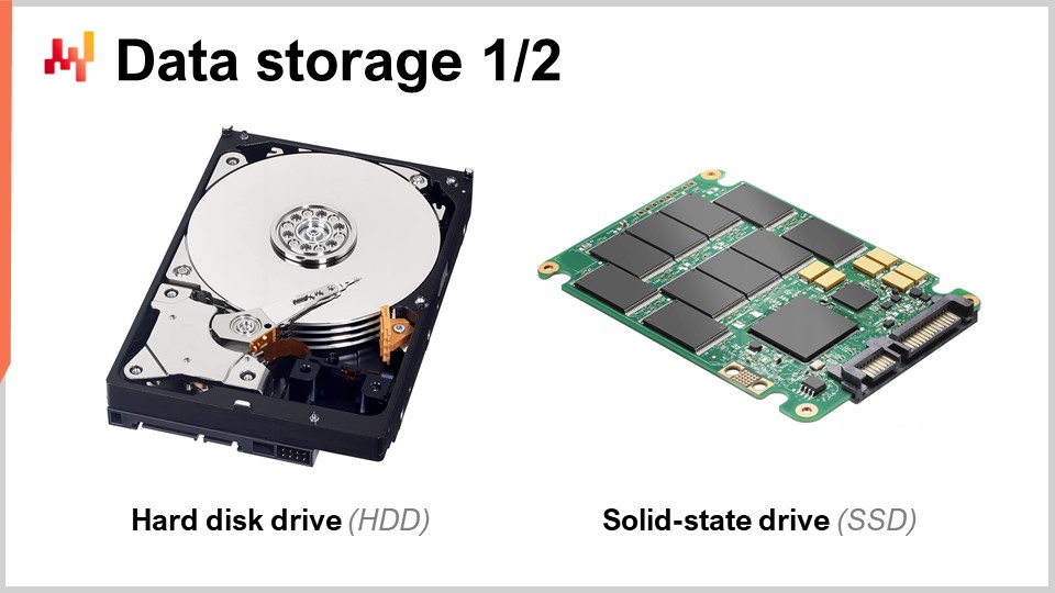
Now, let’s have a look at data storage, which is about persistent data storage. Essentially, you have two classes of widespread data storage. The first one is hard disk drives (HDD) or rotational disks. The second one is solid-state drives (SSD). The interesting thing is that the latency on rotational disks is terrible, and when you look at this picture, you can easily understand why. These disks literally rotate, and when you want to access any random point of data on the disk, on average, you need to wait for half a rotation of the disk. Considering that the very top-end disks are rotating at about 10,000 rotations per minute, it means that you have a built-in three-millisecond latency that cannot be compressed. It’s literally the time it takes for the disk to rotate and to be able to read the precise point of interest on the disk. It’s mechanical and will not improve any further.
HDDs are terrible in terms of latency, but they also have another problem, which is power consumption. As a rule of thumb, an HDD and an SSD both consume about three watts per hour per device. That’s typically the ballpark status quo at present day. However, when the hard drive is running, even if you’re not actively reading anything from the hard drive, you will be consuming three watts just because you need to keep the disk spinning. Reaching 10,000 rotations per minute takes a lot of time, so you need to keep the disk spinning all the time, even if you’re using the disk very infrequently.
On the other hand, when it comes to solid-state drives, they consume three watts when you access them, but when you don’t access the data, they almost don’t consume any power. They have a residual power consumption, but it’s exceedingly small, in the order of milliwatts. This is very interesting because you can have tons of SSDs; if you’re not using them, you don’t pay for the power that they consume. The entire industry has been gradually transitioning from HDDs to SSDs over the last decade.
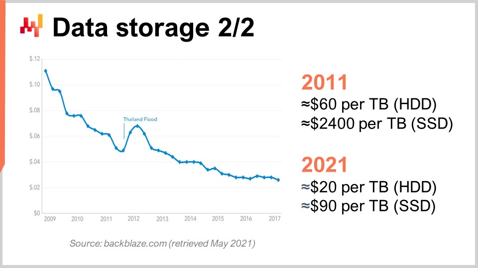
To understand this, we can look at this curve. What we see is that the price per gigabyte of both HDDs and SSDs has been going down over the last couple of years. However, the price is now plateauing. The data is a tiny bit old, but it didn’t vary that much over the last couple of years. During the last 10 years, we see that a decade ago, SSDs were extremely expensive at $2,400 per terabyte, while hard drives were only $60 per terabyte. However, at present day, the price of hard drives has been divided by three, essentially at $20 per terabyte. The price of SSDs has been divided by more than 25, and the trend of decreasing SSD prices is not stopping. SSDs are right now, and probably for the decade to come, the component that is progressing the most, and that’s very interesting.
By the way, I told you that the design of modern compute devices (CPU, GPU, TPU) were essentially two-dimensional with at most 20 layers. However, when it comes to SSDs, the design is increasingly three-dimensional. The most recent SSDs have something like 176 layers. We are reaching, in terms of order, 200 layers. Due to the fact that those layers are incredibly thin, it is not unreasonable to expect that in the future, we have devices with thousands of layers and potentially orders of magnitude more storage capabilities. Obviously, the trick will be that you won’t be able to access all this data all the time, again, due to dark silicon and power dissipation.
It turns out that if you play it nice, a lot of data is accessed very infrequently. SSDs involve a very specific hardware design that comes with tons of quirks, such as the fact that you can only turn bits on but not off. Essentially, imagine you have initially all zeros; you can turn a zero into a one, however, you can’t turn this one into a zero locally. If you want to do that, you have to reset the whole block that can be as large as eight megabytes, which means that when you’re writing, you can turn bits from zero to one, but not from one to zero. In order to turn bits from one to zero, you need to flush the entire block and rewrite it, which leads to all sorts of problems known as write amplification.
During the last decade, SSD drives have internally a layer called the flash translation layer that can mitigate for you all those problems. These flash translation layers are getting better and better over time. However, there are large opportunities to improve further, and in terms of enterprise software, it means that you really want to optimize your design to make the most of SSDs. SSDs are already a much better deal than DRAM when it comes to storing data, and if you play it smartly, you can expect, one decade from now, orders of magnitude of gain that will be earned through the progress of the hardware industry, which is not the case as far as DRAM is concerned.
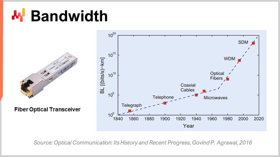
Finally, let’s talk about bandwidth. Bandwidth is probably the most solved problem in terms of technology. However, even if bandwidth can be achieved, we can achieve the sort of bandwidths that are absolutely insane at present date. Commercially, the telecom industry is very complex, and there are tons of problems, so that end consumers don’t actually see all the benefits of the progress that has been made in terms of optical communications.
In terms of optical communication with fiber optic transceivers, the progress is absolutely insane. It’s probably one of those things that are progressing like CPUs were progressing in the ’80s or ’90s. Just to give you an idea, with wavelength division multiplexing (WDM) or space division multiplexing (SDM), now we can reach literally a tenth of terabytes of data transferred per second on a single cable of optic fiber. This is absolutely enormous. We are reaching the point where a single cable can carry enough data to essentially feed an entire data center. What is even more impressive is that the telecom industry has been able to develop new transceivers that can deliver these absolutely crazy performances based on old cables. You don’t even have to deploy new fiber in the streets or physically; you can literally take the fiber that was deployed a decade ago, deploy the new transceiver, and have several orders of magnitude more bandwidth on the very same cable.
The interesting thing is that there is a general law of optical communications: every decade, the distance shrinks at which it becomes interesting to replace electrical communication with optical communications. If we go a few decades back, two decades ago, it took something like 100 meters for optical communication to surpass electrical communication. So if you had distances shorter than 100 meters, you would go for copper; if you had more than 100 meters, you would go for fiber. However, nowadays, with the latest generation, we can have a distance where optics are winning even as short as three meters. If we look one decade ahead, I would not be surprised if we see situations where optical communications are winning even if we are looking at distances as short as half a meter. This means that at some point, I will not be surprised if computers themselves have optical pathways inside, just because it’s more performant than electrical pathways.
From an enterprise software perspective, this is also very interesting because it means that if you’re looking ahead, bandwidth is going to decrease in cost massively. This is substantially subsidized by companies like Netflix, which have dramatic bandwidth consumption. It means that in order to cheat with latency, you could do things like grabbing tons of data preemptively towards the user and then letting the user interact with data that has been brought closer to them with much shorter latency. Even if you bring data that is not needed, what kills you is latency, not bandwidth. It’s better to say, “I have doubts about what sort of data will be needed; I can take a thousand times more data than what I really need, just bring it closer to the end user, let the user or the program interact with this data, and minimize the round trip, and I will be gaining in terms of performance.” This again has a profound impact on the sort of architectural decisions that are made today because they will condition whether you can gain performance with the progress of this class of hardware a decade from now.
In conclusion, latency is the big battle of our time in terms of software engineering. This is really conditioning all the sorts of performance that we have and that will be. Performance is absolutely key because it will not only drive the IT cost, but it will also drive the productivity of the people that operate in your supply chain. Ultimately, that will also drive the performance of the supply chain itself because if you don’t have this performance, you can’t even implement a sort of numerical recipe that would really be smart and deliver deliver advanced optimization and predictive optimization events are what we seek. However, across the board, this battle for better performance is not being won, at least not in the realm of enterprise software. New systems can be, and frequently are, slower than the old ones. This is an acute problem. Slower software performance generates staggering costs for companies that fall for it.
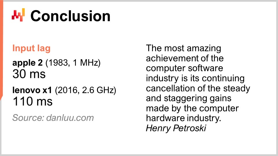
Just to give you an example, it should not be considered a given that better computing hardware gives you better performance. Some people on the internet decided to measure the input latency, or input lag, which is the time it takes after a key press for the corresponding letter to be displayed on the screen. With an Apple II in 1983, which had a 1 MHz processor, the time it took was 30 milliseconds. In 2016, with a Lenovo X1, equipped with a 2.6 GHz processor, a very nice notebook, the latency turned out to be 110 milliseconds. So we have computing hardware that is several thousand times better, yet we end up with latency that is almost four times slower. This is characteristic of what happens when you don’t have mechanical sympathy and don’t pay attention to the computing hardware you have. If you antagonize computing hardware, it repays you with poor performance.
The problem is very real. My suggestion is, when you start looking at any piece of enterprise software for your company, whether it’s open-source or not, remember the elements of mechanical sympathy you’ve learned today. Look at the software and think hard about whether it embraces the deep trends of computing hardware or if it ignores them altogether. If it ignores them, it means that not only will the performance not improve over time, but most likely, it will get worse. Most of the improvements nowadays are achieved through specialization rather than clock speed. If you miss this highway, you’re taking a path that will become slower and slower over time. Avoid these solutions because they usually result from early key design decisions that cannot be undone. You’re stuck with them forever, and it will only get worse year after year. Think a decade ahead when you start looking at these angles.
Now let’s have a look at the questions. That was a fairly long lecture, but it is a challenging topic.
Question: What is your opinion on quantum computers and their utility to tackle complex supply chain optimization problems?
A very interesting question. I registered for the beta of IBM’s quantum computer 18 months ago, when they opened access to their quantum computer in the cloud. My feeling is that it is thrilling, as experts can see all the S-curves flattening but don’t see the new curves appearing out of nowhere. Quantum computing is one of those. However, I believe quantum computers present very tough challenges as far as supply chains are concerned. First, as I said, the battle of our time in terms of enterprise software is latency, and quantum computers don’t do anything about that. Quantum computers give you up to potentially 10 orders of magnitude of speed-up for super tight compute problems. So, quantum computers would be the next stage beyond TPUs, where you can have super tight operations done incredibly fast.
This is very interesting, but to be honest, right now, there are very few companies, to my knowledge, that are even managing to leverage superscalar instructions inside their enterprise software. That means the entire market is leaving a 10 to 28-speed-up on the table that is superscalar GPUs. There are very few people in the supply chain world doing it; maybe Lokad, maybe not. TPUs, I think there is literally nobody. Google is doing it extensively, but I’m not aware of anybody who has ever used TPUs for anything supply chain related. Quantum processors would be the stage beyond TPUs.
I’m definitely very attentive to what is happening with quantum computers, but I believe this is not the bottleneck we face. It’s thrilling because we revisit the von Neumann design established about 70 years ago, but this is not the bottleneck that we or the supply chain will be facing for the next decade. Beyond that, your guess is as good as mine. Yes, it could potentially change everything or not.
Question: Cloud and SaaS offerings are enabling organizations to leverage and convert fixed costs. Are the companies offering such services also working toward reducing their fixed cost and associated risk?
Well, it depends. If I am a cloud computing platform and I sell you processing power, is it really in my interest to make your enterprise software as efficient as possible? Not really. I’m selling you virtual machines, gigabytes of bandwidth, and storage, so actually, quite the opposite. My interest is to make sure that you have software that is as inefficient as possible, so you consume and pay-as-you-go for a crazy amount of resources.
Internally, big tech companies like Microsoft, Amazon, and Google are incredibly aggressive when it comes to the optimization of their computing resources. But they are also aggressive when they are on the front line to pay the bill when they charge a client for renting a virtual machine. If the client is renting a virtual machine that is 10x bigger than what it should be just because the piece of enterprise software they are using is vastly inefficient, it’s not in their interest to interrupt the client’s mistake. It’s just fine for them; it’s good business. When you think that system integrators and cloud computing platforms tend to work hand in hand as partners, you can realize that these categories of people don’t necessarily have your best interest in mind. Now, when it comes to SaaS, it’s kind of different. Indeed, if you end up paying a SaaS provider per user, then it is in the interest of the company, and that’s the case for Lokad, for example. We don’t charge by the computing resources that we consume; we typically charge our clients according to flat monthly fees. Thus, SaaS providers tend to be very aggressive when it comes to their own consumption of compute resources.
However, beware there is a bias: if you are a SaaS company, you can be quite reluctant to do something that would be much nicer for your clients but much more costly in terms of hardware for yourself. It’s not all good and rosy. There is a kind of conflict of interest that impacts all SaaS providers that operate in the supply chain space. For example, they could invest in re-engineering all their systems to deliver better latency and faster webpages, but the thing is, it costs resources, and their clients are not naturally going to pay them more if they do that.
The problem tends to be amplified when it comes to enterprise software. Why is that? It’s because the person who buys the software is typically not the person who uses it. That’s why so much of the enterprise system is incredibly slow. The person who buys the software does not suffer as much as a poor demand planner or inventory manager who has to cope with a super slow system every single day of the year. So there is another angle that is specific to the realm of enterprise software. You really need to analyze the situation, looking at all the incentives that are at play, and when dealing with enterprise software, there are usually plenty of conflicting incentives.
Question: How many times has Lokad had to revisit its approach, given the progress in hardware observed? Can you mention an example, if possible, to just put this content in context of real problems solved?
Lokad, I believe, extensively re-engineered our technology stack about half a dozen times. However, Lokad was founded in 2008, and we had half a dozen major rewrites of the whole architecture. It’s not because the software had progressed that much; the software had progressed, yes, but what drove most of our rewrites was not the fact that the hardware had progressed that much. It was more like we had gained understanding in the hardware. Everything that I’ve presented today was essentially known to the people who were already paying attention a decade ago. So, you see, there is, yes, hardware evolving, but this is very slow, and most of the trends are very predictable, even one decade ahead. This is a long game being played.
Lokad had to undergo massive rewrites, but it was more a reflection that we were gradually becoming less incompetent. We were gaining competency, and so we had a better understanding of how to embrace hardware, rather than the fact that the hardware had been changing the task. It was not always true; there were specific elements that really were game-changing for us. The most notable one was SSDs. We transitioned from HDD to SSD, and it was a complete game changer in our performance, with massive impacts on our architecture. In terms of very concrete examples, the whole design of Envision, the domain-specific programming language that Lokad provides, is based on the insights we gathered at the hardware level. It’s not just one achievement; it’s about doing everything you can think of just faster.
You want to process a table with a billion lines and 100 columns, and you want to do it 100 times faster with the same computing resources? Yes, you can do it. You want to be able to do joins between very large tables with minimal computing resources? Yes, again. Can you have super complex dashboards with literally a hundred tables displayed to the end user in less than 500 milliseconds? Yes, we achieved that. These are mundane achievements, but it’s because we achieved all those that we can put fairly fancy predictive optimization recipes in production. We need to make sure that all the steps that took us there are done with very high productivity.
The biggest challenge when you want to do something very fancy for supply chain in terms of numerical recipes is not the “make it work” stage. You can take college students and achieve a series of prototypes that will deliver some kind of supply chain performance improvement in a matter of weeks. You just take Python and whatever random open-source machine learning library of the day, and those students, if they are smart and willing, will produce a working prototype in a matter of weeks. However, you will never get that into production at scale. That’s the problem. It’s about how you get through all those maturity stages of “make it right,” “make it fast,” and “make it cheap.” That’s where hardware affinity really shines and your capacity to iterate.
There is no single achievement. However, everything that we do, for example when we say Lokad is doing probabilistic forecasting, doesn’t require that much processing power. What really requires processing power is to leverage very extensive distributions of probabilities and to look at all those possible futures and combine all those possible futures with all the possible decisions you can take. That way, you can pick the best ones with financial optimization, which gets very costly. If you don’t have something that is very optimized, you’re stuck. The very fact that Lokad can use probabilistic forecasting in production is a testament that we had extensive hardware-level optimization all the way through the pipelines for all our clients. We are serving about 100 companies nowadays.
Question: Is it better to have an in-house server for enterprise software (ERP, WMS) rather than using cloud services to avoid latency?
I would say nowadays, it doesn’t matter because most of the latencies you experience are within the system. This is not the problem of latency between your user and the ERP. Yes, if you have very poor latency, you might add about 50 milliseconds of latency. Obviously, if you have an ERP, you don’t want to have it sitting in Melbourne while you are operating in Paris, for example. You want to keep the data center close to where you’re operating. However, modern cloud computing platforms have dozens of data centers, so there’s not much difference in terms of latency between in-house hosting and cloud services.
Typically, in-house hosting doesn’t mean placing the ERP on the floor in the middle of the factory or warehouse. Instead, it means putting your ERP into a data center where you’re renting computing hardware. I believe there’s no practical difference between in-house hosting and cloud computing platforms from the perspective of modern cloud computing platforms with data centers all over the globe.
What really makes a difference is whether you have an ERP that internally minimizes all the round trips. For example, what typically kills the performance of an ERP is the interaction between the business logic and the relational database. If you have hundreds of back-and-forth interactions to display a web page, your ERP is going to be terribly slow. So, you need to consider enterprise software designs that do not come with a massive number of round trips. This is an inner property of the enterprise software you’re looking at, and it doesn’t depend much on where you locate the software.
Question: Do you think we need new programming languages that would embrace new hardware design at the core level, using hardware architecture features to their full extent?
Yes, and yes. But full disclosure, I have a conflict of interest here. This is precisely what Lokad has done with Envision. Envision was born from the observation that it is tricky to leverage all the processing power available in modern computers, but it should not be if you design the programming language itself with performance in mind. You can make it supernatural, and that’s why, in the lecture 1.4 about programming paradigms for supply chain, I said if you pick the right programming paradigms, such as array programming or data frame programming, and construct a programming language that embraces those concepts, you get performance almost for free.
The price you pay is that you’re not as expressive as a programming language like Python or C++, but if you’re willing to accept reduced expressiveness and cover all the use cases relevant to supply chain, then yes, you can achieve massive performance improvements. That’s my belief, and that’s why I also stated that, for example, object-oriented programming from the perspective of supply chain optimization brings nothing to the table.
On the contrary, this is a sort of paradigm that only antagonizes the underlying computing hardware. I’m not saying that object-oriented programming is all bad; that’s not what I’m saying. I’m saying that there are areas of software engineering where it makes complete sense, yet it doesn’t make sense as far as predictive optimization of supply chain is concerned. So yes, very much yes, we need programming languages that really embrace that.
I know that I tend to repeat this, but Python was essentially engineered in the late 80s, and they kind of missed everything there was to be seen about modern computers. They have something where, by design, they cannot leverage multi-threading. They have this global lock, so they can’t leverage multiple cores. They can’t leverage locality. They have late binding that really complicates memory accesses. They are very variable, so they consume a lot of memory, which means it is going to play against the cache, etc.
These are the sorts of problems where, if you use Python, it means that you’re going to face uphill battles for the coming decades, and the battle will only get worse over time. They won’t get any better.
The next lecture will be three weeks from now, on the same day of the week, at the same time. It will be at 3 PM Paris time, on the 9th of June. We are going to discuss modern algorithms for supply chain, which is kind of the counterpart of modern computers for supply chain. See you next time.
