00:18 Introduction
02:18 Background
12:08 Why optimize? 1/2 Forecasting with Holt-Winters
17:32 Why optimize? 2/2 - Vehicle routing problem
20:49 The story so far
22:21 Auxiliary Sciences (recap)
23:45 Problems and solutions (recap)
27:12 Mathematical optimization
28:09 Convexity
34:42 Stochasticity
42:10 Multi-objective
46:01 Solver design
50:46 Deep (Learning) lessons
01:10:35 Mathematical optimization
01:10:58 “True” programming
01:12:40 Local search
01:19:10 Stochastic gradient descent
01:26:09 Automatic differentiation
01:31:54 Differential programming (circa 2018)
01:35:36 Conclusion
01:37:44 Upcoming lecture and audience questions
Description
Mathematical optimization is the process of minimizing a mathematical function. Nearly all the modern statistical learning techniques - i.e. forecasting if we adopt a supply chain perspective - rely on mathematical optimization at their core. Moreover, once the forecasts are established, identifying the most profitable decisions also happen to rely, at its core, on mathematical optimization. Supply chain problems frequently involve many variables. They are also usually stochastic in nature. Mathematical optimization is a cornerstone of a modern supply chain practice.
Full transcript
Welcome to this series of supply chain lectures. I’m Joannes Vermorel, and today I will be presenting “Mathematical Optimization for Supply Chain.” Mathematical optimization is the well-defined, formalized, computationally tractable way of identifying the best solution for a given problem. All forecasting problems can be seen as mathematical optimization problems. All decision-making situations in supply chain and outside supply chains can also be seen as mathematical optimization problems. Actually, the mathematical optimization perspective is so anchored in our modern view of the world that it has become very difficult to define the verb “to optimize” outside the very little box that is given to us by the mathematical optimization paradigm.
Now, the literature on the scientific literature on mathematical optimization is vast, and so is the software ecosystem that delivers tools for mathematical optimization. Unfortunately, most of it is of very little use and relevance as far as supply chain is concerned. The goal of this lecture will be twofold: first, we want to understand how to even approach mathematical optimization to get something that is valuable and of practical use from a supply chain perspective. The second element will be to identify, in this vast landscape, some of the most valuable elements there are to be found.
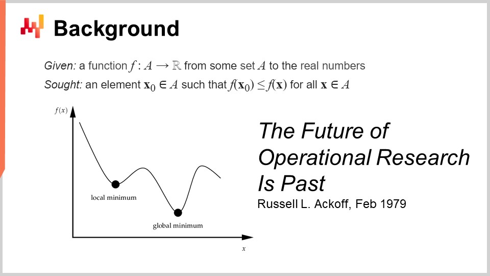
The formal definition of mathematical optimization is straightforward: you think of a function that is typically going to be called the loss function, and this function is going to be real-valued, so it produces just numbers. What you want is to identify the input (X0) that represents the best value that minimizes the loss function. This is typically the mathematical optimization paradigm, and it is deceptively simple. We will see that there are plenty of things that can be said about this general perspective.
This field, I believe, when we think in terms of applied mathematical optimization, was primarily developed under the name of operational research, which we define more specifically as the classic operational research that went from the 1940s to the late 1970s in the 20th century. The idea is that classic operational research, compared to mathematical optimization, really cared about business problems. Mathematical optimization cares about the general form of the optimization problem, much less about whether the problem has any kind of business significance. On the contrary, classic operational research was essentially doing optimization, but not on any kind of problems – on problems that were identified as being of importance for businesses.
Interestingly enough, we went from operational research to mathematical optimization pretty much the same way we went from forecasting, which emerged at the beginning of the 20th century as a field concerned with the general forecasting of future economic activity levels, typically associated with time series forecasts. This domain was essentially superseded by machine learning, which cared more broadly about making predictions on a much broader scope of problems. We could say that we have loosely had the same sort of transition from operational research to mathematical optimization as it was from forecasting to machine learning. Now, when I said that the classic era of operational research went until the late 70s, I had a very specific date in mind. In February 1979, Russell Ackoff published a stunning paper titled “The Future of Operational Research is Past.” To understand this paper, which I believe to be really a landmark in the history of optimization science, you have to understand that Russell Ackoff is essentially one of the founding fathers of operational research.
When he published this paper, he was not a young man anymore; he was 60 years old. Ackoff was born in 1919 and had spent pretty much his entire career working on operational research. When he published his paper, he basically stated that operational research had failed. Not only did it not deliver results, but interest in the industry was dwindling, so there was less interest at the end of the 90s than there was in the field 20 years ago.
The thing that is very interesting to understand is that the cause is absolutely not the fact that the computers at the time were much weaker than the ones we have today. The problem has nothing to do with the limitation in terms of processing power. This is the end of the 70s; computers are very modest compared to what we have nowadays, but they can still deliver millions of arithmetic operations in a reasonable time frame. The problem is not related to the limitation of processing power, especially at a time where processing power is progressing incredibly fast.
By the way, this paper is a fantastic read. I really suggest to the audience to have a look; you can easily find it with your favorite search engine. This paper is very accessible and well written. Although the sort of problems that Ackoff points out in this paper still resonates very strongly four decades down the road, in many ways, the paper is very prescient of many of the problems that are still plaguing present-day supply chains.
So, what is the problem then? The problem is that this paradigm, where you take a function and optimize it, you can prove that your optimization process identifies some good or maybe optimal solution. However, how do you prove that the loss function that you are actually optimizing bears any interest for the business? The problem is that when I say we can optimize a given problem or a given function, what if what you’re optimizing is actually a fantasy? What if this thing has nothing to do with the reality of the business that you’re trying to optimize?
Here lies the crux of the problem, and here lies the reason why those early attempts essentially all failed. It’s because it turned out that when you conjure up some kind of mathematical expression that is supposed to represent the interest of the business, what you obtain is a mathematical fantasy. That’s literally what Russell Ackoff is pointing out in this paper, and he is at a point in his career where he has been playing this game for a very long time and recognizes that it is essentially leading nowhere. In his paper, he shares the view that the field has failed, and he proposes his diagnosis, but he doesn’t have much of a solution to offer. It’s very interesting because one of the founding fathers, a very respected and recognized researcher, says that this entire field of research is a dead end. He will spend the rest of his life, which is still quite long, transitioning entirely from a quantitative perspective on business optimization toward a qualitative perspective. He will spend the last three decades of his life going for qualitative methods and still produce very interesting work in the second part of his life after this turning point.
Now, as far as this series of lectures is concerned, what do we do because the points that Russell Ackoff is raising about operational research remain very valid nowadays? Actually, I have already started to address the biggest problems that Ackoff was pointing out, and at the time, he and his peers didn’t have solutions to offer. They could diagnose the problem, but they didn’t have a solution. In this series of lectures, the solutions I’m proposing are of a methodological nature, just like the fact that Ackoff points out that there is a deep methodological problem with this operational research perspective.
The methods I propose are essentially twofold: on one side, the supply chain personnel, and on the other side, the method titled experimental optimization that happens to be really complementary to mathematical optimization. Also, I am positioning, unlike operational research that claims to be of business interest or business relevance, the way I’m approaching the problem today is not through the angle or the lenses of operational research. I’m approaching the problem through the lenses of mathematical optimization, which I position as a pure auxiliary science for supply chain. I say that there is nothing intrinsically fundamental about mathematical optimization for supply chain; it is just of foundational interest. It is just a means, not an end. That’s where it differs. The point may be very simple, but it has great importance when it comes to actually achieving prediction-grade results with the whole thing.
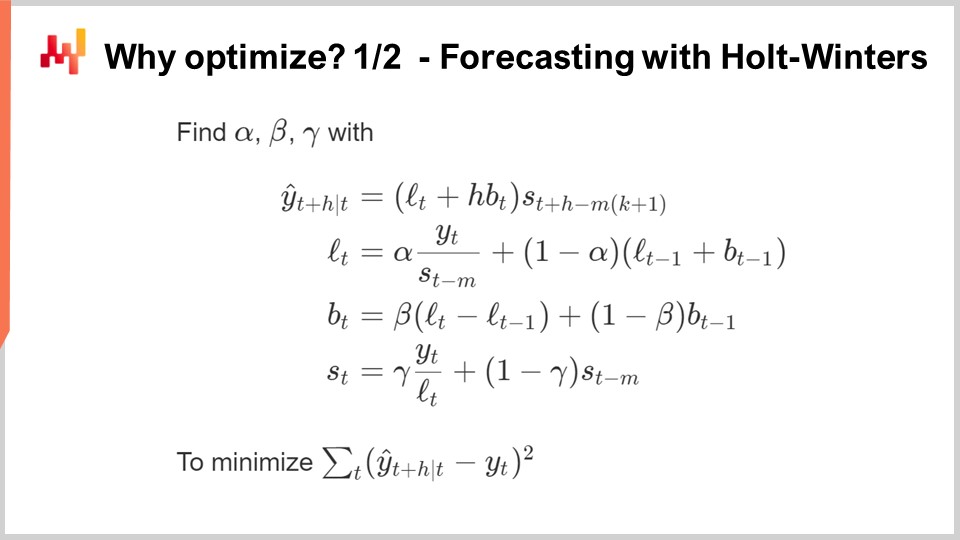
Now, why do we want to even optimize in the first place? Most forecasting algorithms have a mathematical optimization problem at their core. On this screen, what you can see is the very classic multiplicative Holt-Winters time series forecasting algorithm. This algorithm is primarily of historical interest; I would not recommend any present-day supply chain to actually leverage this specific algorithm. But for the sake of simplicity, this is a very simple parametric method, and it is so concise that you can actually put it entirely on one screen. It’s not even that verbose.
All the variables you can see on the screen are just plain numbers; there are no vectors involved. Essentially, Y(t) is your estimate; this is your time series forecast. Here on the screen, it’s going to be forecasting H periods ahead, so H is like the horizon. And you can think that you’re actually working on Y(t), which is essentially your time series. You can think of a weekly aggregated sales data or monthly aggregated sales data. This model has essentially three components: it has Lt, which is the level (you have one level per period), Bt, which is the trend, and St, which is a seasonal component. When you say that you want to learn the Holt-Winters model, you have three parameters: alpha, beta, and gamma. These three parameters are essentially just numbers between zero and one. So, you have three parameters, all numbers between zero and one, and when you say that you want to apply the Holt-Winters algorithm, it just means that you will identify the proper values for those three parameters, and that’s it. The idea is that these parameters, alpha, beta, and gamma, are going to be the best if they minimize the sort of error that you’ve specified for your forecast. On this screen, you can see a mean squared error, which is very classic.
The point about mathematical optimization is to conjure a method to do this identification of the right parameter values for alpha, beta, and gamma. What can we do? Well, the easiest and most simplistic method is something like grid search. Grid search would say that we are just going to explore all the values. Because these are fractional numbers, there is an infinite number of values, so we are actually going to pick a resolution, let’s say steps of 0.1, and we’ll go in increments of 0.1. Since we have three variables between 0 and 1, we go in 0.1 increments; that’s about 1,000 iterations to go through and identify the best value, considering this resolution.
However, this resolution is pretty weak. 0.1 gives you about a 10% resolution on the sort of scale that you have for your parameters. So maybe you want to go for 0.01, which is much better; that’s a 1% resolution. However, if you do that, the number of combinations really explodes. You go from 1,000 combinations to a million combinations, and you see that’s the problem with grid search: very quickly, you hit a combinatorial wall, and you have an enormous number of options.
Mathematical optimization is about conjuring algorithms that give you more bang for your buck for a given amount of computing resources that you want to throw at the problem. Can you get a much better solution than just brute search? The answer is yes, absolutely.
So what can we do in this case to actually get a better solution with investing fewer computational resources? First, we could use some kind of gradient. The whole expression for Holt-Winters is completely differentiable, except for one single division that is a tiny edge case that is relatively easy to take care of. So, this entire expression, including the loss function, is entirely differentiable. We could use a gradient to guide our search; that would be one approach.
Another approach would say that in practice, in supply chain, you maybe have tons of time series. So maybe instead of treating every single time series independently, what you want to do is a grid search for the first 1,000 time series, and you’re going to invest, and then you’re going to identify combinations for alpha, beta, and gamma that are good. Then, for all the other time series, you will just pick from this shortlist of candidates to identify the best solution.
You see, there are plenty of simple ideas on how you can actually do vastly better than just going for a pure grid search approach, and the essence of mathematical optimization, and then all sorts of decision-making problems can also be seen typically as mathematical optimization problems.
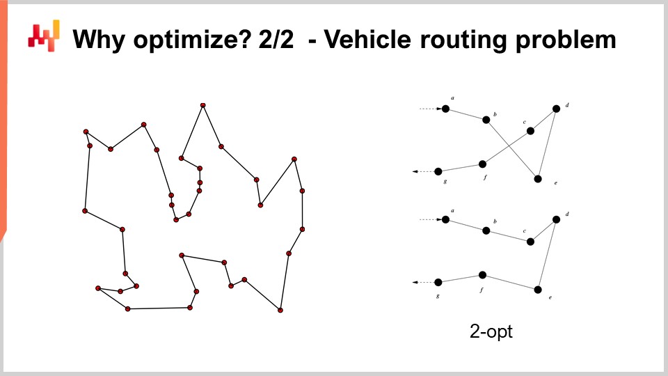
For example, the vehicle routing problem that you can see on the screen can be seen as a mathematical optimization problem. It is about picking the list of points. I did not write down the formal version of the problem because it’s relatively variable and doesn’t bring much insight to the table. But if you want to think about it, you can just think, “I have points, I can assign a kind of pseudo-rank that is just a score to every single point, and then I have an algorithm that sorts all the points by pseudo-ranks in ascending order, and that’s my route.” The goal of the algorithm will be to identify the values for those pseudo-ranks that give you the best routes.
Now, with this problem, we see that we have a problem where suddenly grid search is not even remotely an option. We have dozens of points, and if we were to try all the combinations, that would be way too large. Also, the gradient is not going to help us, at least it’s not obvious how it’s going to help us, because the problem is very discrete in nature, and there is not something that is like an obvious gradient descent for this sort of problem.
However, it turns out that if we want to approach this sort of problem, there are very powerful heuristics that have been identified in the literature. For example, the two-opt heuristic, published by Croes in 1958, gives you a very straightforward heuristic. You start with a random route, and in this route, whenever the route crosses over itself, you apply a permutation to remove the crossing. So, you start with a random route, and the first crossing that you observe, you do the permutation to remove the crossing, and then rinse and repeat. You repeat the process with the heuristic until you have no crossing left. What you will get out of this very simple heuristic is actually a very good solution. It may not be optimal in the true mathematical sense, so it’s not necessarily the perfect solution; however, it is a very good solution, and you can get that with a relatively minimal amount of computational resources.
The problem with the two-opt heuristic is that it’s a very fine heuristic, but it’s incredibly specific to this one problem. What is really of interest for mathematical optimization is to identify methods that work on large classes of problems instead of having one heuristic that is just going to work for one specific version of a problem. So, we want to have very general methods.
Now, the story so far in this lecture series: this lecture is part of a series of lectures, and this present chapter is dedicated to the auxiliary sciences of supply chain. In the first chapter, I presented my views on supply chain both as a field of study and as a practice. The second chapter was dedicated to methodology, and in particular, we introduced one methodology that is of utmost relevance to the present lecture, which is experimental optimization. That is the key to addressing the very valid problem identified by Russell Ackoff decades ago. The third chapter is entirely dedicated to supply chain personnel. In this lecture, we focus on identifying the problem we are about to solve, as opposed to mixing together the solution and the problem. In this fourth chapter, we are investigating all the auxiliary sciences of supply chain. There is a progression from the lowest level in terms of hardware, moving up to the level of algorithms, and then to mathematical optimization. We are progressing in terms of levels of abstraction throughout this series.
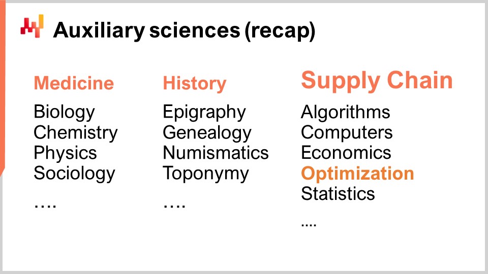
Just a brief recap on auxiliary sciences: they offer a perspective on supply chain itself. The present lecture is not about supply chain per se, but rather one of the auxiliary sciences of supply chain. This perspective makes a significant difference between the classic operational research perspective, which was supposed to be an end, as opposed to mathematical optimization, which is a means to an end but not an end in itself, at least as far as supply chain is concerned. Mathematical optimization doesn’t care about business specifics, and the relationship between mathematical optimization and supply chain is similar to the relationship between chemistry and medicine. From a modern perspective, you don’t have to be a brilliant chemist to be a brilliant physician; however, a physician who claims to know nothing about chemistry would seem suspicious.
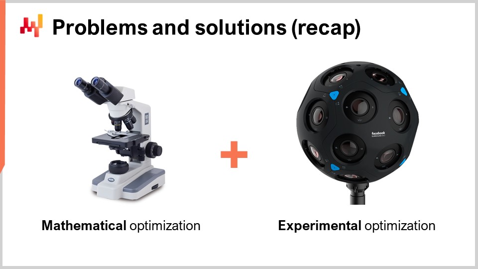
Mathematical optimization assumes that the problem is known. It doesn’t care about the validity of the problem, but rather focuses on making the most of what you can for a given problem in terms of optimization. In a way, it is like a microscope – very powerful but with an incredibly narrow focus. The danger, as we go back to the discussion of the future of operational research, is that if you point your microscope in the wrong place, you might become distracted by interesting but ultimately irrelevant intellectual challenges.
That’s why mathematical optimization needs to be used in conjunction with experimental optimization. Experimental optimization, which we covered in the previous lecture, is the process by which you can iterate with feedback from the real world towards better versions of the problem itself. Experimental optimization is a process to mutate not the solution but the problem, so that iteratively you can converge towards a good problem. This is the crux of the matter, and where Russell Ackoff and his peers at the time didn’t have a solution. They had the tools to optimize a given problem, but not the tools to mutate the problem until the problem was good. If you take a mathematical problem as you can write it in your ivory tower, without feedback from the real world, what you get is a fantasy. Your starting point, when you begin an experimental optimization process, is just a fantasy. It takes the feedback of the real world to make it work. The idea is to go back and forth between mathematical optimization and experimental optimization. At every stage of your experimental optimization process, you will use mathematical optimization tools. The goal is to minimize both computational resources and engineering efforts, allowing the process to iterate towards the next version of the problem.
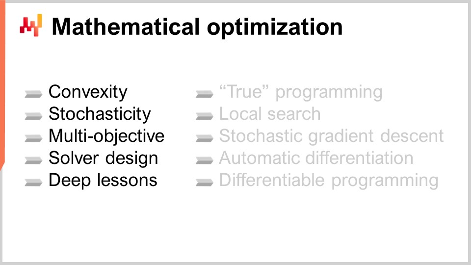
In this lecture, we will first refine our understanding of the mathematical optimization perspective. The formal definition is deceptively simple, but there are complexities we need to be aware of to achieve practical relevance for supply chain purposes. We will then explore two broad classes of solvers that represent the state of the art in mathematical optimization from a supply chain perspective.
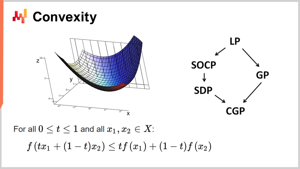
First, let’s discuss convexity and early works in mathematical optimization. Operational research initially focused on convex loss functions. A function is said to be convex if it abides by certain properties. Intuitively, a function is convex if, for any two points on the manifold defined by the function, the straight line connecting those points will always be above the values taken by the function in between those points.
Convexity is key to allowing true mathematical optimization, where you can prove results. Intuitively, when you have a convex function, it means that for any point of the function (any candidate solution), you can always look around and find a direction in which you can descend. No matter where you start, you can always descend, and descending is always a good move. The only point where you cannot descend any further is essentially the optimal point. I’m simplifying here; there are edge cases where you have non-unique solutions or no solutions at all. But putting aside a few edge cases, the only point where you cannot optimize further with a convex function is the optimal point. Otherwise, you can always descend, and descending is a good move.
There has been an enormous amount of research on convex functions, and various programming paradigms have emerged over the years. LP stands for linear programming, and other paradigms include second-order conic programming, geometric programming (dealing with polynomials), semi-definite programming (involving matrices with positive eigenvalues), and geometric conic programming. These frameworks all have in common that they deal with structured convex problems. They are convex both in their loss function and in the constraints that restrict eligible solutions.
These frameworks have been of very high interest, with an intense scientific literature produced. However, despite their impressive-sounding names, these paradigms have very little expressiveness. Even simple problems exceed the capabilities of these frameworks. For example, the optimization of the Holt-Winters parameters, a basic forecasting model from the 1960s, already exceeds what any of these frameworks can do. Similarly, the vehicle routing problem and the traveling salesman problem, both of which are simple problems, exceed the capabilities of these frameworks.
That’s why I was saying at the very beginning that there has been an enormous body of literature, but there is very little use. The only point where you cannot descend any further is essentially the optimal point. I’m simplifying here; there are edge cases where you have non-unique solutions or no solutions at all. But putting aside a few edge cases, the only point where you cannot optimize further with a convex function is the optimal point. Otherwise, you can always descend, and descending is a good move.
There has been an enormous amount of research on convex functions, and various programming paradigms have emerged over the years. LP stands for linear programming, and other paradigms include second-order conic programming, geometric programming (dealing with polynomials), semi-definite programming (involving matrices with positive eigenvalues), and geometric conic programming. These frameworks all have in common that they deal with structured convex problems. They are convex both in their loss function and in the constraints that restrict eligible solutions.
These frameworks have been of very high interest, with an intense scientific literature produced. However, despite their impressive-sounding names, these paradigms have very little expressiveness. Even simple problems exceed the capabilities of these frameworks. For example, the optimization of the Holt-Winters parameters, a basic forecasting model from the 1960s, already exceeds what any of these frameworks can do. Similarly, the vehicle routing problem and the traveling salesman problem, both of which are simple problems, exceed the capabilities of these frameworks.
That’s why I was saying at the very beginning that there has been an enormous body of literature, but there is very little use. One part of the problem was a misguided focus on the pure mathematical optimization kind of solvers. These solvers are very interesting from a mathematical perspective because you can produce mathematical proofs, but they can only be used with literally toy problems or completely made-up problems. Once you are in the real world, they fail, and there has been very little progress in these fields for the last few decades. As far as the supply chain is concerned, almost nothing, except a few niches, have any relevance to these solvers.
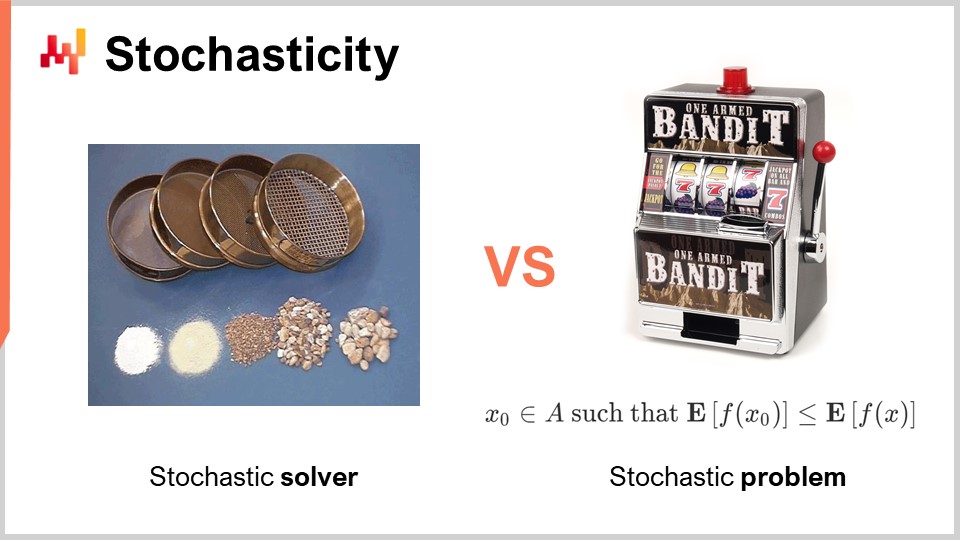
Another aspect, which was entirely dismissed and ignored during the classic era of operational research, is randomness. Randomness or stochasticity is of critical importance in two radically different ways. The first way we need to approach randomness is in the solver itself. Nowadays, all the state-of-the-art solvers extensively leverage stochastic processes internally. This is very interesting as opposed to having a fully deterministic process. I am talking about the inner workings of the solver, the piece of software that implements the mathematical optimization techniques.
The reason why all state-of-the-art solvers extensively leverage stochastic processes has to do with the way modern computing hardware exists. The alternative to randomness when exploring solutions is to remember what you have done in the past, so you do not get stuck in the same loop. If you have to remember, you will consume memory. The problem lies in the fact that we need to do a lot of memory accesses. One way to introduce randomness is usually a way to largely alleviate the need for random memory access.
By making your process stochastic, you can avoid probing your own database of what you have tested or not tested among possible solutions for the problem you want to optimize. You do it a bit randomly, but not completely. This has key importance in practically all modern solvers. One of the somewhat counterintuitive aspects of having a stochastic process is that although you can have a stochastic solver, the output can still be fairly deterministic. To understand this, consider the analogy of a series of sieves. A sieve is fundamentally a physical stochastic process, where you apply random movements and the sieving process takes place. Although the process is completely stochastic, the outcome is completely deterministic. At the end, you get a completely predictable outcome out of the sieving process, even though your process was fundamentally random. This is exactly the sort of thing that happens with well-engineered stochastic solvers. This is one of the key ingredients of modern solvers.
Another aspect, which is orthogonal when it comes to randomness, is the stochastic nature of the problems themselves. This was mostly absent from the classic era of operational research – the idea that your loss function is noisy and that any measurement you are going to get of it will have some degree of noise. This is almost always the case in supply chain. Why? The reality is that in supply chain, whenever you are taking a decision, it is because you anticipate some kind of future events. If you decide to buy something, it is because you anticipate that there will be a need for it later on in the future. The future is not written, so you can have some insights about the future, but the insight is never perfect. If you decide to produce a product now, it is because you expect that later on in the future there will be demand for this product. The quality of your decision, which is producing today, depends on future uncertain conditions, and thus any decision you take in supply chain will have a loss function that varies depending on these future conditions that cannot be controlled. The sort of randomness due to dealing with future events is irreducible, and that is of key interest because it means that we are fundamentally dealing with stochastic problems.
However, if we go back to the classic mathematical solvers, we see that this aspect is completely absent, which is a big problem. It means that we have classes of solvers that cannot even comprehend the sort of problems we will face, because the problems that will be of interest, where we want to apply mathematical optimization, will be of a stochastic nature. I am talking about the noise in the loss function.
There is an objection that if you have a stochastic problem, you can always transform it back into a deterministic problem through sampling. If you evaluate your noisy loss function 10,000 times, you can have an approximately deterministic loss function. However, this approach is incredibly inefficient because it introduces a 10,000-fold overhead on your optimization process. The mathematical optimization perspective is about getting the best results for your limited computational resources. It is not about investing an infinitely large amount of computational resources to solve the problem. We have to deal with a finite amount of computational resources, even if this amount is fairly large. Thus, when looking at solvers later on, we have to keep in mind that it is of primary interest to have solvers that can natively apprehend stochastic problems instead of defaulting to the deterministic approach.
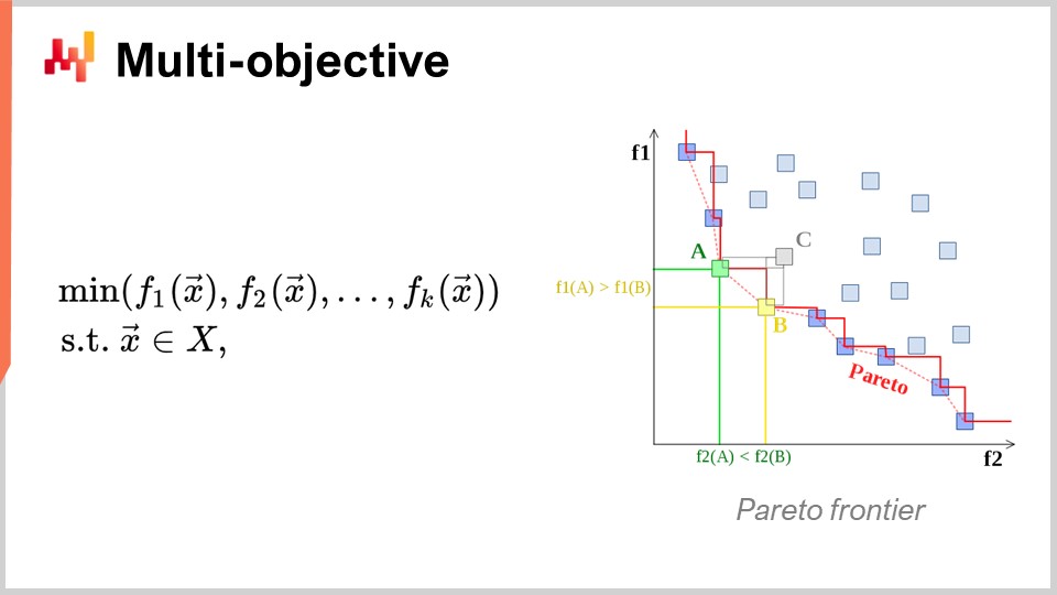
Another angle, which is also of primary interest, is multi-objective optimization. In the naive expression of the mathematical optimization problem, I said that the loss function was essentially single-valued, so we had one value that we wanted to minimize. But what if we have a vector of values, and what we want to do is to find the solution that gives the lowest point according to the lexicographical order of all the vectors, like f1, f2, f3, etc.?
Why is this even of interest from a supply chain perspective? The reality is that if you adopt this multi-objective perspective, you can express all your constraints as just one dedicated loss function. You can first have a function that counts your constraints violation. Why do you have constraints in supply chain? Well, you have constraints all over the place. For example, if you place a purchase order, you have to make sure that you have enough space in your warehouse to store the goods when they arrive. So, you have constraints on storage space, production capacity, and more. The idea is that, instead of having a solver where you have to special case the constraints, it is more interesting to have a solver that can deal with multi-objective optimization and where you can express the constraints as one of the objectives. You just count the number of constraint violations, and you want to minimize that, bringing this number of violations to zero.
The reason why this mindset is very much relevant for supply chain is because the optimization problems that supply chains face are not cryptographic puzzles. These are not the super tight combinatorial problems where either you have a solution and it’s good, or you are just one bit off the solution and you have nothing. In supply chain, obtaining what is typically called a feasible solution – a solution that satisfies all the constraints – is typically completely trivial. Identifying one solution that satisfies the constraints is not a big undertaking. What is very difficult is, among all the solutions that satisfy the constraints, identifying the one that is most profitable for the business. This is where it becomes very difficult. Finding a solution that does not violate the constraints is very straightforward. This is not the case in other fields, for example, in mathematical optimization for industrial design, where you want to do component placement inside a cell phone. This is an incredibly tightly constrained problem, and you can’t cheat by giving up on one constraint and having a little bump on your cell phone. It’s a problem that is incredibly tight and combinatorial, and where you really need to treat constraints as a first-class citizen. This is not necessary, I believe, for the vast majority of supply chain problems. Thus, it is again of very high interest to have techniques that can deal with multi-objective optimization natively.

Now, let’s discuss a little bit more about the design of the solver. From a very high-level perspective on how we want to engineer a piece of software that is going to produce solutions for a very broad class of problems, there are two very notable design aspects that I would like to put forward. The first aspect to consider is whether we are going to operate on a white box or black box perspective. The idea of a black box perspective is that we can process any arbitrary program, so the loss function can be any arbitrary program. We don’t care; we treat that as a complete black box. The only thing we want is a program where we can evaluate the program and get the value of a tentative solution. On the contrary, a white box approach emphasizes the fact that the loss function itself has a structure that we can inspect and leverage. We can see inside the loss function. By the way, when I was discussing convexity a few slides before, all those models and pure mathematical solvers were really white box approaches. They are the extreme case of white box approaches, where not only can you see inside the problem, but the problem has a very rigid structure, such as semi-definite programming, where the form is very narrow. However, without going for something as rigid as a mathematical framework, you can, for example, say that as part of the white box, you have something like the gradient that will help you. A gradient of the loss function is of key interest because suddenly you can know in which direction you want to go to descend, even if you don’t have a convex problem where the simple gradient descent guarantees a good result. As a rule of thumb, if you can white box your solver, you will have a solver that is orders of magnitude more performant compared to a black box solver.
Now, as a second aspect, we have offline versus online solvers. The offline solver typically operates in batch, so an offline solver is just going to take the problem, execute, and you will have to wait until it completes. At this point in time, when the solver completes, it gives you the best solution or something that is the best identified solution. On the contrary, an online solver works much more with a best-effort approach. It’s going to identify a solution that is passable and then invest computational resources to iterate toward better and better solutions as time passes and as you invest more computational resources. What is really of key interest is that when you approach a problem with an online solver, it means that you can pretty much pause the process at any point in time and get an early candidate solution. You can even resume the process. If we go back to the mathematical solvers, they are typically batch solvers where you have to wait until the end of the process.
Unfortunately, operating in the supply chain world can be a very bumpy ride, as covered in one of the previous lectures of this series. There will be situations where usually you can afford to spend, let’s say, three hours to run this mathematical optimization process. But sometimes, you can have IT glitches, real-world problems, or an emergency in your supply chain. In such cases, it will be a lifesaver if what was usually taking three hours can be interrupted after five minutes and provide an answer, even a bad one, as opposed to no answer at all. There is a saying in the army that the worst plan is no plan, so it’s better to have a very rough plan rather than nothing at all. This is exactly what an online solver gives you. These are the key design elements that we will be keeping in mind in the following discussion.
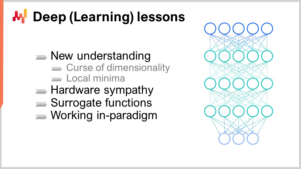
Now, to conclude this first section of the lecture about approaching mathematical optimization, let’s have a look at the deep learning lessons. Deep learning has been a complete revolution for the field of machine learning. However, at its core, deep learning also has a mathematical optimization problem. I believe that deep learning generated a revolution within mathematical optimization itself and completely changed the way we look at optimization problems. Deep learning redefined what we consider as the state of the art of mathematical optimization.
Nowadays, the largest deep learning models are dealing with more than a trillion parameters, which is a thousand billion. Just to put that in perspective, most of the mathematical solvers struggle to even deal with 1,000 variables and typically collapse with only a few tens of thousands of variables, no matter how much computing hardware you throw at them. In contrast, deep learning succeeds, arguably using a large amount of computational resources, but nonetheless, it is feasible. There are deep learning models in production that have over a trillion parameters, and all those parameters are optimized, which means that we have mathematical optimization processes that can scale to a trillion parameters. This is absolutely stunning and radically different from the performance we saw with classic optimization perspectives.
The interesting thing is that even problems that are completely deterministic, like playing Go or chess, which are non-statistical, discrete, and combinatorial, have been most successfully solved with methods that are completely stochastic and statistical. This is puzzling because playing Go or chess can be seen as discrete optimization problems, yet they are solved most efficiently nowadays with methods that are completely stochastic and statistical. This goes against the intuition the scientific community had about these problems two decades ago.
Let’s revisit the understanding that has been unlocked by deep learning concerning mathematical optimization. The first thing is to completely revisit the curse of dimensionality. I believe that this concept is mostly flawed, and deep learning is proving that this concept is not how you should even think about the difficulty of an optimization problem. It turns out that when you look at classes of mathematical problems, you can prove mathematically speaking that certain problems are exceedingly hard to solve perfectly. For example, you’ve ever heard of NP-hard problems, you know that as you add dimensions to the problem, it becomes exponentially more difficult to solve. Each extra dimension makes the problem harder, and there is a cumulative barrier. You can prove that no algorithm can ever hope to solve the problem perfectly with a limited amount of computational resources. However, deep learning showed that this perspective was mostly flawed.
First, we have to differentiate between the representational complexity of the problem and the intrinsic complexity of the problem. Let me clarify these two terms with an example. Let’s have a look at the time series forecasting example given initially. Let’s say we have a sales history, daily aggregated over three years, so we have a time vector daily aggregated of about 1,000 days. This is the representation of the problem.
Now, what if I transition to a time series representation by the second? This is the same sales history, but instead of representing my sales data in daily aggregates, I’m going to represent this time series, the very same time series, in per second aggregates. That means there are 86,400 seconds in every single day, so I’m going to inflate the size and dimension of my representation of the problem by 86,000.
But if we start thinking about the intrinsic dimension, it is not because I have a sales history, and it’s not because I go from a per day aggregation to a per second aggregation, that I am increasing the complexity or the dimensional complexity of the problem by 1,000. Most likely, if I go into sales aggregated per second, the time series is going to be incredibly sparse, so it’s going to be mostly zeros for practically all the buckets. I am not increasing the interesting dimensionality of the problem by a factor of 100,000. Deep learning clarifies that it’s not because you have a representation of the problem with many dimensions that the problem is fundamentally hard.
Another angle associated with dimensionality is that although you can prove that certain problems are NP-complete, for example, the traveling salesman problem (a simplified version of the vehicle routing problem presented at the beginning of this lecture), the traveling salesman is technically what is known as an NP-hard problem. So, it’s a problem where if you want to find the best solution in the general case, it is going to be exponentially costly as you add points to your map. But the reality is that these problems are very easy to solve, as illustrated with the two-opt heuristic; you can get excellent solutions with a minimal amount of computational resources. So, beware that mathematical proofs, demonstrating that some problems are very hard, can be deceptive. They don’t tell you that if you’re okay having an approximate solution, the approximation can be excellent, and sometimes it’s not even an approximation; you’re going to get the optimal solution. It’s just that you can’t prove it’s optimal. This doesn’t say anything about whether you can approximate the problem, and very frequently, those problems supposedly plagued by the curse of dimensionality are straightforward to solve because their interesting dimensions are not that high. Deep learning has successfully demonstrated that many problems thought to be incredibly difficult were not that difficult in the first place.
The second key insight was local minima. The majority of researchers working on mathematical optimization and operational research went for convex functions because there were no local minima. For a long time, people not working on convex functions were thinking about how to avoid being stuck in a local minimum. Most of the efforts were devoted to working on things like meta-heuristics. Deep learning has provided a renewed understanding: we don’t care about local minima. This understanding comes from recent work originating from the deep learning community.
If you have a very high dimension, you can show that local minima vanish as the dimension of the problem increases. Local minima are very frequent in low-dimensional problems, but if you increase the dimension of the problems to hundreds or thousands, statistically speaking, local minima become incredibly improbable. To the point where, when looking at very large dimensions like millions, they vanish completely.
Instead of thinking that a higher dimension is your enemy, as was associated with the curse of dimensionality, what if you could do the exact opposite and inflate the dimension of the problem until it becomes so great that it’s trivial to have a clean descent with no local minima whatsoever? It turns out that this is exactly what is being done in the deep learning community and with models that have a trillion parameters. This approach gives you a very clean way to gradient your way forward.
Essentially, the deep learning community showed that it was irrelevant to have a proof about the quality of descent or the ultimate convergence. What matters is the speed of descent. You want to iterate and descend very rapidly toward a very good solution. If you can have a process that descends faster, you will ultimately go further in terms of optimization. These insights go against the general understanding of mathematical optimization, or what was the mainstream understanding two decades ago.
There are other lessons to be taken from deep learning, as it is a very rich field. One of them is hardware sympathy. The problem with mathematical solvers, such as conic programming or geometric programming, is that they focus on mathematical intuition first and not on the computing hardware. If you design a solver that fundamentally antagonizes your computing hardware, no matter how smart your math may be, chances are that you’re going to be desperately inefficient due to poor use of the computational hardware.
One of the key insights of the deep learning community is that you have to play nice with the computing hardware and design a solver that embraces it. This is why I started this series of lectures on auxiliary sciences for supply chain with modern computers for supply chain. It’s important to understand the hardware you have and how to make the best use of it. This hardware sympathy is how you can achieve models with one trillion parameters, granted it requires a large cluster of computers or a supercomputer.
Another lesson from deep learning is the use of surrogate functions. Traditionally, mathematical solvers aimed to optimize the problem as it was, without deviating from it. However, deep learning showed that sometimes it’s better to use surrogate functions. For example, very frequently for predictions, deep learning models use cross-entropy as the error metric instead of mean square. Practically nobody in the real world is interested in cross-entropy as a metric, as it is quite bizarre.
So why are people using cross-entropy? It provides incredibly steep gradients, and as deep learning showed, it’s all about the speed of descent. If you have very steep gradients, you can descend very rapidly. People might object and say, “If I want to optimize mean square, why should I use cross-entropy? It’s not even the same target.” The reality is that if you optimize cross-entropy, you will have very steep gradients, and in the end, if you evaluate your solution against mean square, you will get a better solution according to the mean square criterion as well, very frequently, if not always. I’m just simplifying for the sake of this explanation. The idea of surrogate functions is that the true problem is not an absolute; it’s just something that you will use for control to assess the final validity of your solution. It is not necessarily something that you will be using while the solver is in progress. This goes completely against the ideas involved with the mathematical solvers that were popular during the last couple of decades.
Finally, there is the importance of working in paradigms. With mathematical optimization, there is implicitly a division of labor involved in organizing your engineering workforce. The implicit division of labor attached to mathematical solvers is that you will have mathematical engineers on one side, who are responsible for engineering the solver, and problem engineers on the other side, whose responsibility is to express the problem in a form suitable for processing by the mathematical solvers. This division of labor was prevalent, and the idea was to make it as simple as possible for the problem engineer, so they only have to express the problem in the most minimalistic and purest fashion, letting the solver do the job.
Deep learning showed that this perspective was deeply inefficient. This arbitrary division of labor was not the best way to approach the problem at all. If you do that, you end up with situations that are impossibly difficult, meaning vastly exceeding the state of the art for whoever are the mathematical engineers working on the optimization problem. A much better way is to have the problem engineers put in some extra effort to reframe the problems in ways that make them much more suitable for optimization by the mathematical optimizer.
Deep learning is about a set of recipes that allow you to frame the problem on top of your solver, so you get the most out of your optimizer. Most of the developments in the deep learning community have been focused on crafting these recipes that are very good at learning while playing well within the paradigm of the solvers they have (e.g., TensorFlow, PyTorch, MXNet). The conclusion is that you really want to collaborate with the problem engineer, or in supply chain terminology, the supply chain scientist.
Now let’s move on to the second and last section of this lecture about the most valuable elements of the literature. We will have a look at two broad classes of solvers: local search and differentiable programming.
First, let me pause again on the term “programming.” This word has critical importance because, from a supply chain perspective, we really want to be able to express the problem that we face, or the problem that we think we are facing. We don’t want some kind of super low-resolution version of the problem that just happens to fit some semi-absurd mathematical hypothesis, such as needing to express your problem in a cone or something like that. What we’re really interested in is having access to a true programming paradigm.
Remember, those mathematical solvers like linear programming, second-order conic programming, and geometric programming all came with a programming keyword. However, over the last couple of decades, what we expect from a programming paradigm has evolved dramatically. Nowadays, we want something that lets you deal with almost arbitrary programs, programs in which you have loops, branches, and possibly memory allocations, etc. You really want something as close as possible to an arbitrary program, not some kind of super limited toy version that has some interesting mathematical properties. In supply chain, it’s better to be approximately correct rather than exactly wrong.
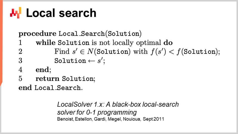
To deal with generic optimization, let’s start with local search. Local search is a deceptively simple mathematical optimization technique. The pseudocode involves starting with a random solution, which you represent as a pack of bits. You then initialize your solution randomly and start flipping bits randomly to explore the neighborhood of the solution. If, through this random exploration, you find a solution that happens to be better, this becomes your new reference solution.
This surprisingly powerful approach can work with literally any program, treating it as a black box, and can also restart from any known solution. There are plenty of ways to make this approach better. One way is differential computation, not to be confused with differentiable computation. Differential computation is the idea that if you execute your program on a given solution and then flip one bit, you can re-execute the same program with a differential execution, without having to re-execute the whole program. Obviously, your mileage may vary, and it very much depends on the structure of the problem. One way to speed up the process is not to leverage some kind of extra information about the black box program that we operate, but just be able to speed up the program itself, still treating it mostly as a black box, because you don’t re-execute the whole program every single time.
There are other approaches to make local search better. You can improve the sort of moves that you make. The most basic strategy is called the k-flips, where you flip a number k of bits with k being a very small number, something like a couple to a dozen. Instead of just flipping bits, you can let the problem engineer state the sort of mutations to apply to the solution. For example, you may express that you want to apply some sort of permutation in your problem. The idea is that these smart moves often preserve the satisfaction of some constraints in your problem, which can help the local search process converge faster.
Another way to improve local search is to not explore the space completely at random. Instead of flipping bits randomly, you can try to learn the right directions, identifying the most promising areas for flips. Some recent papers have shown that you can plug a tiny deep learning module on top of the local search, acting as a generator. However, this approach can be tricky in terms of engineering, as you have to ensure that the overhead introduced by the machine learning process yields a positive payback in terms of computational resources.
There are other well-known heuristics, and if you want a very good synthetic view of what it takes to implement a modern local search engine, you can read the paper “LocalSolver: A Black-Box Local-Search Solver for 0-1 Programs.” The company that operates LocalSolver also has a product with the same name. In this paper, they give an engineering outlook at what is going on under the hood in their production-grade solver. They use multi-start and simulated annealing for better results.
One caveat I would add on local search is that it doesn’t deal very well or natively with stochastic problems. With stochastic problems, it’s not as easy as simply saying “I have a better solution,” and immediately deciding that it becomes the best solution. It is more tricky than that, and you need to put in some extra effort before jumping to the solution assessed as the new best.
Now, let’s move toward the second class of solvers that we’ll be discussing today, which is differentiable programming. But first, to understand differentiable programming, we need to comprehend stochastic gradient descent. Stochastic gradient descent is an iterative, gradient-based optimization technique. It emerged as a series of techniques pioneered in the early 1950s, making it almost 70 years old. It remained fairly niche for almost six decades, and we had to wait for the advance of deep learning to realize the true potential and power of stochastic gradient descent.
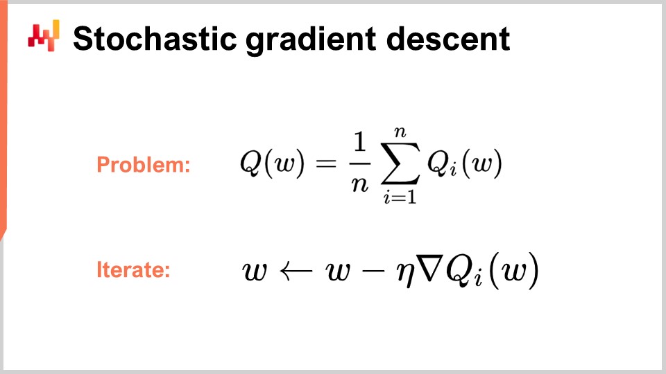
Stochastic gradient descent assumes that the loss function can be decomposed additively into a series of components. In the equation, Q(W) represents the loss function, which is decomposed into a series of partial functions, Qi. This is relevant because most learning problems can be viewed as having to learn a prediction based on a series of examples. The idea is that you can decompose your loss function as the average error committed over the entire dataset, with a local error for each data point. Many supply chain problems can also be decomposed additively in this manner. For example, you can decompose your supply chain network into a series of performances for every single SKU, with a loss function attached to each SKU. The true loss function you want to optimize is the total.
When you have this decomposition in place, which is very natural for learning problems, you can iterate with the stochastic gradient descent (SGD) process. The parameter vector W can be a very large series, as the largest deep learning models have a trillion parameters. The idea is that at every step of the process, you update your parameters by applying a small amount of gradient. Eta is the learning rate, a small number typically between 0 and 1, often around 0.01. Nabla of Q is the gradient for a partial loss function Qi. Surprisingly, this process works well.
SGD is said to be stochastic because you randomly pick your next i element, jumping through your dataset and applying a tiny bit of gradient to your parameters at every single step. This is the essence of stochastic gradient descent.
It remained relatively niche and largely ignored by the community at large for almost six decades, because it’s quite surprising that stochastic gradient descent works at all. It works because it provides an excellent trade-off between the noise in the loss function and the computational cost of accessing the loss function itself. Instead of having a loss function that needs to be assessed against the entire dataset, with stochastic gradient descent, we can take one data point at a time and still apply a little bit of gradient. This measurement is going to be very fragmentary and noisy, yet this noise is actually okay because it is very fast. You can perform orders of magnitude more tiny, noisy optimizations compared to processing the entire dataset.
Surprisingly, the noise introduced helps the gradient descent. One of the problems in high-dimensional spaces is that local minima become relatively inexistent. However, you can still face large areas of plateaus where the gradient is very small, and the gradient descent doesn’t have a direction to pick for descent. The noise gives you steeper, more noisy gradients that help with descent.
What is also interesting with gradient descent is that it is a stochastic process, but it can deal with stochastic problems for free. If Qi is a stochastic function with noise and gives a random result that varies each time you evaluate it, you don’t even need to change a single line of the algorithm. Stochastic gradient descent is of prime interest because it gives you something that is completely aligned with the paradigm that is relevant for supply chain purposes.
The second question is: where does the gradient come from? We have a program, and we just take the gradient of the partial loss function, but where does this gradient come from? How do you get a gradient for an arbitrary program? It turns out there is a very elegant, minimalistic technique discovered a long time ago called automatic differentiation.
Automatic differentiation emerged in the 1960s and was refined over time. There are two types: forward mode, discovered in 1964, and reverse mode, discovered in 1980. Automatic differentiation can be seen as a compilation trick. The idea is that you have a program to compile, and with automatic differentiation, you have your program that represents the loss function. You can recompile this program to get a second program, and the output of the second program is not the loss function but the gradients of all the parameters involved in the calculation of the loss function.
Furthermore, automatic differentiation gives you a second program with compute complexity basically identical to that of your initial program. This means that not only do you have a way to create a second program that computes the gradients, but also the second program has the same compute characteristics in terms of performance as the first program. It’s a constant factor inflation in terms of compute cost. The reality, however, is that the second program obtained doesn’t have exactly the same memory characteristics as the initial program. Although the fine print goes beyond the scope of this present lecture, we can discuss that during the questions. Essentially, the second program, called the reverse, is going to require more memory, and in some pathological situations, it can require much more memory than the initial program. Remember that more memory creates problems with compute performance, as you cannot assume uniform memory access.
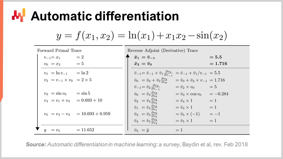
To illustrate a bit what automatic differentiation looks like, as I mentioned, there are two modes: forward and reverse. From a learning perspective or supply chain optimization perspective, the only mode of interest to us is the reverse mode. What you can see on the screen is a loss function F, completely made up. You can see the forward trace, a sequence of arithmetic or elementary operations that take place to compute your function for two given input values, X1 and X2. This gives you all the elementary steps done to compute the final value.
The idea is that for every elementary step, and most of them are just basic arithmetic operations like multiplication or addition, the reverse mode is a program that executes the same steps but in reverse order. Instead of having the forward values, you’re going to have the adjoints. For every arithmetic operation, you will have their reverse counterpart. The transition from the forward operation to the counterpart is very straightforward.
Even if it looks complicated, you have a forward execution and a reverse execution, where your reverse execution is nothing but an elementary transformation applied to every single operation. At the end of the reverse, you get the gradients. Automatic differentiation may look complicated, but it is not. The first prototype we implemented was less than 100 lines of code, so it is very straightforward and essentially a cheap transpilation trick.
Now, this is interesting because we have stochastic gradient descent, which is a fantastically powerful optimization mechanism. It is incredibly scalable, online, whiteboard, and works natively with stochastic problems. The only problem that was left is how to obtain the gradient, and with automatic differentiation, we have the gradient for a fixed overhead or constant factor, for pretty much any arbitrary program. What we get in the end is differentiable programming.
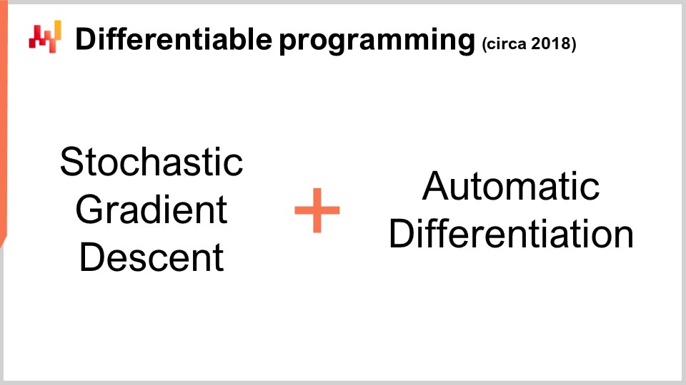
Interestingly enough, differentiable programming is a combination of stochastic gradient descent and automatic differentiation. Although these two techniques, stochastic gradient descent and automatic differentiation, are decades old, differentiable programming only rose to prominence in early 2018 when Yann LeCun, the Head of AI at Facebook, began to communicate about this concept. LeCun did not invent this concept, but he was instrumental in making it popular.
For example, the deep learning community initially used backpropagation rather than automatic differentiation. For those familiar with neural networks, backpropagation is a complex process that is orders of magnitude more complicated to implement than automatic differentiation. Automatic differentiation is superior in all aspects. With this insight, the deep learning community refined its vision of what constitutes learning in deep learning. Deep learning combined mathematical optimization with various learning techniques, and differentiable programming emerged as a clean concept that isolated the non-learning parts of deep learning.
Modern deep learning techniques, such as the transformer model, assume a differentiable programming environment operating underneath. This allows researchers to focus on the learning aspects that are built on top. Differentiable programming, while foundational to deep learning, is also highly relevant for supply chain optimization and supporting supply chain learning processes, such as statistical forecasting.
Just like with deep learning, there are two parts to the problem: differentiable programming as the base layer and optimization or learning techniques on top of that. The deep learning community aims to identify architectures that work well with differentiable programming, such as transformers. Similarly, one must identify the architectures that work well for optimization purposes. This is what has been done to learn how to play Go or Chess in highly combinatorial settings. We will discuss techniques that work well for supply chain-specific optimization in later lectures.
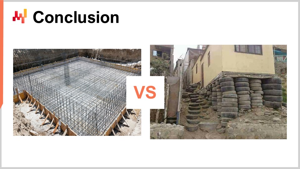
But now, it’s time to conclude. A fair share of the supply chain literature and even most of its software implementations are quite confused when it comes to mathematical optimization. This aspect is usually not even properly identified as such, and as a result, practitioners, researchers, and even software engineers working for enterprise software companies often blend into their numerical recipes fairly haphazardly when it comes to mathematical optimization. They have a big problem, as one component has not been identified as being of a mathematical optimization nature, and because people are not even aware of what is available in the literature, they often resort to crude grid searches or hasty heuristics that yield erratic and inconsistent performance. As a conclusion to this lecture, from now on, whenever you encounter a supply chain numerical method or supply chain software that claims to deliver any kind of analytical feature, you need to ask yourself what is going on in terms of mathematical optimization and what is being done. If you realize that the providers do not offer a crystal clear view about this perspective, the odds are that you are on the left side of the illustration, and this is not the place you want to be.
Now, let’s have a look at the questions.
Question: Is the transition toward computational methods a prerequisite skill in operations, and would operational roles become obsolete, or vice versa?
First, let me clarify a few things. I believe it is a mistake to push these sorts of concerns towards the CIO. People expect way too much from their CIOs. As the Chief Information Officer, you already have to deal with the base layer of your software infrastructure, such as computational resources, low-level transactional systems, network integrity, and cybersecurity. The CIO should not be expected to have an understanding of what it takes to actually do something of value for your supply chain.
The problem is that in many companies, people are so desperately ignorant of anything computer-related that the CIO becomes the go-to person for everything. The reality is that the CIO should deal with the base layer of the infrastructure, and then it’s up to each specialist to address their specific needs with the computational resources and software tools available to them.
Regarding operational roles becoming obsolete, if your role is to manually go through Excel spreadsheets all day long, then yes, your role is very likely to become obsolete. This has been a known issue since 1979 when Russell Ackoff published his paper. The problem is that people knew this method of dealing with decisions was not the future, but it remained the status quo for a very long time. The crux of the problem is that companies need to understand the experimental process. I believe there will be a transition where companies start to reacquire these skills. Many large North American companies after World War II had some knowledge of operations research among their executives. It was a hot new topic, and the boards of large companies knew things about operational research. As Russell Ackoff points out, due to the lack of results, these ideas were pushed down the ladder of the company until they were even outsourced completely, as they were mostly irrelevant and did not deliver tangible results. I believe that operations research will only return if people learn the lessons from why the classic era of operational research did not deliver results. The CIO will have only a modest contribution in this undertaking; it is mostly a matter of rethinking the added value of the people inside the company.
You want to have a capitalistic contribution, and that goes back to one of my previous lectures about product-oriented delivery in the sense of software products for supply chains. The crux is: what sort of capitalistic added value do you deliver to your company? If the answer is none, then you might not be part of what your company should become and will become in the future.
Question: What about using the Excel solver to minimize the MRMSC value and finding the optimal value for alpha, beta, and gamma?
I believe this question is relevant for the Holt-Winters case, where you can actually find a solution with grid search. However, what is happening in this Excel solver? Is it a gradient descent or something else? If you’re referring to the linear solver of Excel, it’s not a linear problem, so Excel cannot do anything for you in that case. If you have some other solvers in Excel or add-ins, yes, they can operate, but this is a very dated perspective. It does not embrace a more stochastic view; the sort of forecast you get is a non-probabilistic forecast, which is a dated approach.
I’m not saying that Excel cannot be used, but the question is, what sort of programming capabilities are being unlocked in Excel? Can you do stochastic gradient descent in Excel? Probably, if you add some dedicated add-in. Excel allows you to plug any arbitrary program on top of it. Could you potentially do differentiable programming in Excel? Yes. Is it a good idea to do it in Excel? No. To understand why, you have to go back to the product-oriented software delivery concept, which details what is going wrong with Excel. It boils down to the programming model and whether you can actually maintain your work over time with a team effort.
Question: Optimization problems are typically skewed toward vehicle routing or forecasting. Why not consider optimizing the entire supply chain as well? Wouldn’t that reduce costs compared to looking at isolated areas?
I completely agree. The curse of supply chain optimization is that when you perform a local optimization on a subproblem, you’re most likely going to displace the problem, not solve it for the entire supply chain. I completely agree, and as soon as you start looking at a more complex problem, you’re dealing with a hybrid problem – for example, a vehicle routing problem combined with a replenishment strategy. The issue is that you need a very generic solver to approach this because you don’t want to be restricted. If you have a very generic solver, you need to have very generic mechanisms instead of relying on smart heuristics like the two-opt, which only works well for vehicle routing and not for something that is a hybrid of both replenishment and vehicle routing at the same time.
In order to transition toward this holistic perspective, you have to not be afraid of the curse of dimensionality. Twenty years ago, people would say that these problems are already exceedingly hard and NP-complete, like the traveling salesman problem, and you want to solve an even more difficult problem by entangling it with another problem. The answer is yes; you want to be able to do that, and that’s why it’s essential to have a solver that lets you deal with arbitrary programs because your resolution may be the consolidation of many entangled and interleaved problems.
Indeed, the idea of solving these problems in isolation is much weaker compared to solving everything. It’s better to be approximately correct than exactly wrong. It’s much better to have a very weak solver that tackles the entire supply chain as a system, as a block, as opposed to having advanced local optimizations that just create problems in other places as you micro-optimize locally. The true optimization of the system is not necessarily the best optimization for every part, so it is natural that if you optimize for the interest of the whole company and its entire supply chain, it’s not going to be locally optimal because you take into account the other aspects of the company and its supply chain.
Question: After carrying out an optimization exercise, when should we revisit the scenario considering that new constraints can appear at any time? The answer is that you should revisit the optimization frequently. This is the role of the supply chain scientist that I’ve presented in the second lecture of this series. The supply chain scientist will revisit the optimization as often as necessary. If a new constraint emerges, like a gigantic ship blocking the Suez Canal, it was unexpected, but you have to deal with this disruption in your supply chain. You don’t have any option but to address these issues; otherwise, the system you’ve put in place will generate nonsensical results because it’s going to operate under false conditions. Even if you don’t have an emergency to deal with, you still want to invest your time to think about the angle most likely to generate the biggest return for the company. This is fundamentally research and development. You have the system in place, it operates, and you’re just trying to identify areas where you can improve the system. It becomes an applied research process that is highly capitalistic and erratic. As a supply chain scientist, there are days when you spend your entire day testing numerical methods, none of which deliver any better results than what you already have. On some days, you do a tiny tweak, and you’re very lucky, saving the company millions. It’s an erratic process, but on average, the outcome can be massive.
Question: What would be the use cases for optimization problems other than linear programming, integer programming, mixed programming, and in the case of Weber and cost of goods?
I would reverse the question: where do you see that linear programming has any relevance to any supply chain problem? There is virtually no supply chain problem that is linear. My objection is that these frameworks are very simplistic and cannot even approach toy problems. As I said, these mathematical frameworks, like linear programming, cannot even approach a toy problem like the hard winter optimization for an ancient, low-dimensional parametric forecasting model. They can’t even deal with the traveling salesman problem or pretty much anything else.
Integer programming or mixed-integer programming is just a generic term for adding that some of the variables are going to be integers, but it doesn’t change the fact that these programming frameworks are just toy mathematical frameworks that are nowhere near the expressiveness needed to tackle supply chain problems.
When you ask about the use cases of optimization problems, I invite you to have a look at all my lectures about supply chain personas. We already have a series of supply chain personas, and I’m listing literally tons of problems that can be approached through mathematical optimization. In the lectures about the supply chain personas, we have Paris, Miami, Amsterdam, and a world series, with more coming. We have lots of problems that need to be approached and would deserve to be approached with a proper mathematical optimization perspective. However, you will see that for every single one of those problems, you will not be able to frame them within the super tight and mostly bizarre constraints that emerge from these mathematical frameworks. Again, those mathematical frameworks are mostly about convexity, and this is not the right perspective for supply chain. Most of the points we deal with are non-convex. But it’s okay; it’s not because they are non-convex that they are impossibly hard. You see, it’s just that you won’t be able to have a mathematical proof at the end of the day. But your boss or your company, they care about profit, not whether you have a mathematical proof to support the decision. They care about the fact that you can take the right decision in terms of production, replenishment, prices, assortments, and whatnot, not that you have a mathematical proof attached to those decisions.
Question: How long should the learning algorithm data be stored for aiding in learning?
Well, I would say, considering that data storage nowadays is incredibly cheap, why not keep it forever? Data storage is so inexpensive; for example, just go to a supermarket, and you can see the price point of a one terabyte hard drive is around 60 or something. So, it’s incredibly cheap.
Now, obviously, there is a separate concern that if you have personal data in your data, then the data you keep becomes a liability. But from a supply chain perspective, if we assume that you’ve expunged all the personal data first, because you typically don’t need to have personal data in the first place. You don’t need to keep credit card numbers around, or the names of your clients. You only need to have client identifiers and whatnot. If you just expunge all the personal data from your data, I would say, how long? Well, keep it forever.
One of the points in supply chain is that you have limited data. It’s not like deep learning problems such as image recognition, where you can process all the images on the web and have access to nearly infinite databases to crunch. In supply chain, your data is always limited. Indeed, if you want to forecast future demand, there are very few industries where looking further than a decade in the past is truly relevant, statistically speaking, to forecast the demand for the next quarter. But nonetheless, I would say it’s always easier to truncate the data if you need it rather than realize that you’ve discarded data and now it’s missing. So my suggestion is to keep everything, expunge personal data, and at the very end of your data pipeline, you will see if it’s better to filter out the very old data. It might be, or it might not be; it depends on the industry you’re operating in. For example, in aerospace, when you have parts and aircraft with an operational lifetime of four decades, having data in your system for the last four decades is of relevance.
Question: Is multi-objective programming a function of two or more objectives, such as the sum or minimizing multiple functions in one goal?
There are multiple variants of how you want to approach multi-objectives. It is not about having a function that is a sum because, if you have the sum, then it’s just a matter of decomposition and structure of the loss function. No, it’s really about having a vector. And indeed, there are essentially multiple flavors of multi-objective programming. The most interesting flavor is the one where you want to go for a lexicographic ordering. As far as supply chain is concerned, the minimization, when you want to say that you take the mean or the max of the many functions, may be of interest, but I’m not too sure. I believe that the multi-objective approach, where you can actually inject constraints and treat the constraints as just part of your regular optimization, is very much of interest for supply chain purposes. The other variants might be interesting as well, but I’m not so sure. I’m not saying they are not; I’m just saying that I’m not sure.
Question: How would you decide when to use an approximate solution against the optimized solution?
I mean, I’m not too sure I understand the question. The idea is that, if there is one lesson from deep learning to be learned, it’s that there is no one optimal solution. Everything is an approximation to a certain degree. Even when you say you have numbers, in computers, numbers do not come with infinite precision; they come with finite precision. And this finite precision can actually, in some circumstances, come back at you and bite you. So the answer is, it’s always approximate. I would say the biggest lesson is that it’s an illusion to think that there is even a perfect solution out there. There is no such thing as a perfect, optimal solution. All the solutions that you have are approximations, and some of them are, I would say, slightly less or more approximate. So, I’m not too sure about the sense of your question, but from the mathematical optimization perspective, it means that you have a loss function to assess the quality, and at the end of the day, if you have two competing solutions, you have your loss function to assess which one is the best. That’s the way it operates.
Question: Why was the time series, in terms of historical data, divided by 86,400 in the first place?
It wasn’t. It was an example. I just wanted to outline and push the situation to an absurd state where you see, when you go for a time series, a classical time series forecasting algorithm, you adopt what is known as an equi-spaced time series. There are plenty of ways to represent time series, and the most typical way to represent the time series is the equi-spaced flavor of time series, where you go for aggregation in buckets of equal length. That’s typically what you get with daily aggregation or weekly aggregation. You have buckets that have the same length, and your series has a nice vector-like structure.
But what I’m pointing out is that it is arbitrary to a large degree. You can decide to represent data as daily data, but you could decide to represent data by the second. Would it ever make sense to represent data by the second? The answer is yes; it depends on the sort of problems. For example, if you are an electricity provider and you want to manage a grid, then you have to manage the power at every second so that you have exactly the balance of the supply of electricity in your grid with the consumption of power. And this balance is actually tuned by the second. So, there might be situations where representing data by the second makes sense. For the sale in your local store, it might not make sense. What I wanted to point out with that 86,400, by the way, is just 24 hours times 60 minutes times 60 seconds, and I wanted to clarify the fact that you always have a representation of your data, and you should not confuse the representation of your data that comes with a certain dimensionality with the intrinsic dimension of your data, which may have a completely different dimension. The representation is, to a large extent, completely made up and arbitrary. It gives you a numerical indicator, such as having three years’ worth of data, so that you have a vector of dimension one thousand. But this one thousand is something that is largely made up because it is based on the decision to aggregate data on a daily basis. If you chose any other alternative period, you would get a different dimension. That’s the point I wanted to make, and that’s what deep learning really got right: to have such other things where you’re not fooled into being confused by arbitrary choices of representation of the data. You want to be kind of representation-agnostic.
Question: By introducing probabilistic forecasting, we transition to a cost function and constraints that are probabilistic in their nature. What implication does it have on the process of finding a solution?
Well, it does have one very basic and fundamental constraint. If you have a solver that cannot process problems, and again, remember that you can always go back from a stochastic problem to a deterministic problem by just averaging out your outcome over a very large number of samples, then you’re kind of in trouble in terms of computational costs. It means that you will have to spend 10,000 times or so more processing power to get to a satisfying solution compared to an alternative solution. The implication is you really want to make sure that your mathematical optimization tooling, the infrastructure that you have, is natively capable of dealing with stochastic problems. That’s exactly what you get with differentiable programming, not so much with local search, but you can enhance or revise local search so that it operates more smoothly in those sorts of situations as well.
Fundamentally, when you go for probabilistic forecasting, it does not just challenge the way you look at the future; it also deeply challenges the sort of tooling and instrumentation that you have to work with those forecasts. That’s exactly the sort of tooling that Lokad has been developing for the last decade. The reason is that we need to have tooling that can work well with the sort of stochastic problems that invariably emerge in supply chain because pretty much all the problems in supply chains have an ingredient of uncertainty, and thus they are all dealing with a stochastic problem to some extent.
Excellent. So, the next lecture will be on the same day of the week, a Wednesday. There will be some vacation between now and then. The next lecture will be on September 22nd, and I hope to see you all. This time, we will be discussing machine learning for supply chain. See you then.
References
- The Future of Operational Research Is Past, Russell L. Ackoff, February 1979
- LocalSolver 1.x: A black-box local-search solver for 0-1 programming, Thierry Benoist, Bertrand Estellon, Frédéric Gardi, Romain Megel, Karim Nouioua , September 2011
- Automatic differentiation in machine learning: a survey, Atilim Gunes Baydin, Barak A. Pearlmutter, Alexey Andreyevich Radul, Jeffrey Mark Siskind, last revised February 2018
