Continuous Ranked Probability Score (CRPS)
Updated by Alexey Tikhonov, May 2024.
Probabilistic forecasts assign a probability to every possible future. Yet, all probabilistic forecasts are not equally accurate, and metrics are needed to assess the respective accuracy of distinct probabilistic forecasts. Simple accuracy metrics such as MAE (Mean Absolute Error) or MAPE (Mean Absolute Percentage Error) are not directly applicable to probabilistic forecasts. The Continuous Ranked Probability Score (CRPS) generalizes the MAE to the case of probabilistic forecasts. Along with the cross entropy, the CPRS is one of the most widely used accuracy metrics where probabilistic forecasts are involved.
Overview
The CRPS is frequently used in order to assess the respective accuracy of two probabilistic forecasting models. In particular, this metric can be combined with a backtesting process in order to stabilize the accuracy assessment by leveraging multiple measurements over the same dataset.
This metric notably differs from simpler metrics such as MAE because of its asymmetric expression: while the forecasts are probabilistic, the observations are deterministic. Unlike the pinball loss function, the CPRS does not focus on any specific point of the probability distribution, but considers the distribution of the forecasts as a whole.
Formal definition
Let $${X}$$ be a random variable.
Let $${F}$$ be the cumulative distribution function (CDF) of $${X}$$, such as $${F(y)=\mathbf{P}\left[X \leq y\right]}$$.
Let $${x}$$ be the observation, and $${F}$$ the CDF associated with an empirical probabilistic forecast.
The CRPS between $${x}$$ and $${F}$$ is defined as:
where $${𝟙}$$ is the Heaviside step function and denotes a step function along the real line that attains:
- the value of 1 if the real argument is positive or zero,
- the value of 0 otherwise.
The CRPS is expressed in the same unit as the observed variable (e.g., if a product’s demand was forecasted in units, CRPS will also be expressed in units).
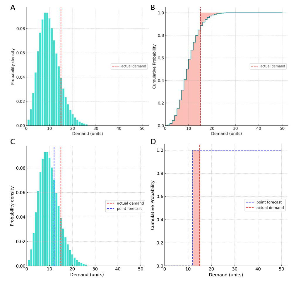
The CRPS generalizes the mean absolute error (MAE). In fact, it reduces to the MAE if the forecast is deterministic. This point is illustrated in chart D below.
Known properties
Gneiting and Raftery (2004) show that the continuous ranked probability score can be equivalently written as:
where
- $${X}$$ and $${X^*}$$ are independent copies of a linear random variable,
- $${X}$$ is the random variable associated with the cumulative distribution function $${F}$$,
- $${\mathbf{E}[X]}$$ is the expected value of $${X}$$.
Numerical evaluation
From a numerical perspective, a simple way of computing CPRS consists of breaking down the original integral into two integrals on well-chosen boundaries to simplify the Heaviside step function, which gives:
In practice, since $$F$$ is an empirical distribution obtained through a forecasting model, the corresponding random variable $${X}$$ has a compact support, meaning that there is only a finite number of points where $${\mathbf{P}[X = x] \gt 0}$$. Also, all values of $$x$$ are discrete numbers. Thus, the integrals can be turned into discrete finite sums as illustrated by the formula below and chart B in the next section.
In the formula (4) an index $$n$$ stands for the last element of the right tail of a probability distribution (e.g. highest demand value having non-zero probability).
Finally, as CRPS computation is performed for one time point, to compute the CRPS over certain evaluation period of interest (e.g., for responsibility window, which is a sum of supplier lead time and reorder period) we should take an average for the respective CRPS values computed for that period.
Visual intuition
To illustrate CRPS computation, consider the following example (consult the charts below):
A: Initially, we built a probabilistic demand forecast using a negative binomial distribution and truncating its tales with probabilities lower than 0.1% (which represents extremely unlikely events, such as those that occur once every three years or so). Predicted demand values with non-zero probabilities spanned the range from 1 to 26 units. Later on, it turned out that the actual demand was 15 units (as depicted by the vertical red dashed line).
B: We computed CRPS according to the 4th formula above (see “Numerical evaluation”). The resulting CRPS value represents the sum of two areas filled with light red color.
C: Same as chart A but with a point forecast added for comparison.
D: CRPS computation applied to the point forecast demonstrates that when CRPS is applied to a point forecast the result is an MAE accuracy metric. Indeed, point forecasts are trivial forms of probabilistic forecasts where we implicitly assign 100% probability to a single value. Then, a cumulative probability chart for CRPS will be represented by two step functions - one for point forecasts and one for actual demand. This means that depending on the relative positions of the point forecast vs. the actual value, one of the two sums in the CRPS formula (4) will turn to zero: the first sum for overpredictions and the second sum for underpredictions.

For the example provided through these 4 charts, the resulting CRPS values for probabilistic forecast and for the point forecast are 3.32 and 3, respectively. Looking at the numbers one might conclude that the point forecast is more accurate because its accuracy metric is smaller (better) than that of the probabilistic forecast. However, this conclusion is wrong.
In the example above we just considered one value of actual demand, however when the probabilistic forecast is learned using historical data, the probabilities are adjusted according to the respective demand values’ frequencies of occurrence (considering the values available in the learning dataset). If they are chosen appropriately, then the average CRPS value for the test dataset will be comparable to the one for the training/validation dataset as the forecast will adequately represent frequencies of occurrence of different demand values in the test data.
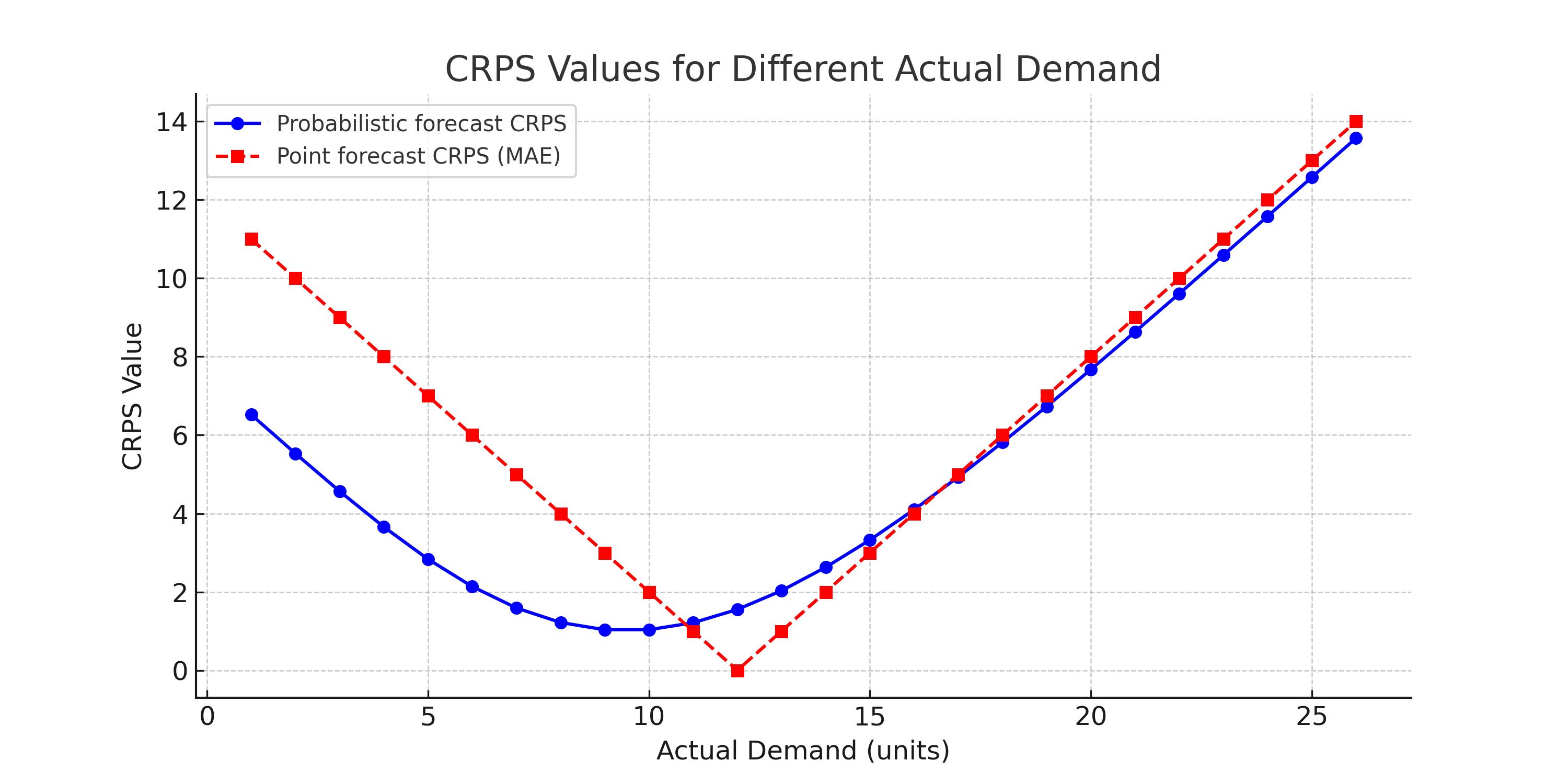
The chart below demonstrates the superiority of probabilistic forecasts relative to point forecasts.

Note how smoothly CRPS changes depending on different actual values. Further note that apart from a tiny region (where the point forecast is very close to the actual), in all other areas CRPS for probabilistic forecasts is smaller that that of the point forecast.
If we had multiple different point forecasts, this observation would still remain true. One would have to mentally move the red curve left or right depending on the point prediction, but the superiority of probabilistic forecasting would still be valid.
References
Gneiting, T. and Raftery, A. E. (2004). Strictly proper scoring rules, prediction, and estimation. Technical Report no. 463, Department of Statistics, University of Washington, Seattle, Washington, USA.