00:19 Introduction
04:33 Two definitions for ‘algorithm’
08:09 Big-O
13:10 The story so far
15:11 Auxiliary sciences (recap)
17:26 Modern algorithms
19:36 Outperforming “optimality”
22:23 Data structures - 1/4 - List
25:50 Data structures - 2/4 - Tree
27:39 Data structures - 3/4 - Graph
29:55 Data structures - 4/4 - Hash table
31:30 Magic recipes - 1/2
37:06 Magic recipes - 2/2
39:17 Tensor comprehensions - 1/3 - The ‘Einstein’ notation
42:53 Tensor comprehensions - 2/3 - Facebook’s team’s breakthrough
46:52 Tensor comprehensions - 3/3 - Supply chain perspective
52:20 Meta techniques - 1/3 - Compression
56:11 Meta techniques - 2/3 - Memoization
58:44 Meta techniques - 3/3 - immutability
01:03:46 Conclusion
01:06:41 Upcoming lecture and audience questions
Description
The optimization of supply chains relies on solving numerous numerical problems. Algorithms are highly codified numerical recipes intended to solve precise computational problems. Superior algorithms mean that superior results can be achieved with fewer computing resources. By focusing on the specifics of supply chain, algorithmic performance can be vastly improved, sometimes by orders of magnitude. “Supply chain” algorithms also need to embrace the design of modern computers, which has significantly evolved over the last few decades.
Full transcript
Welcome to this series of supply chain lectures. I’m Joannes Vermorel, and today I will be presenting “Modern Algorithms for Supply Chain.” Superior compute capabilities are instrumental for achieving superior supply chain performance. More accurate forecasts, more fine-grain optimization, and more frequent optimization are all desirable in order to achieve a superior supply chain performance. There is always a superior numerical method just slightly beyond the computing resources that you can afford.
Algorithms, to keep it simple, make computers go faster. Algorithms are a branch of mathematics, and this is a very active field of research. The progress in this field of research frequently outpaces the progress of computing hardware itself. The goal for this lecture is to understand what modern algorithms are about and, more specifically from a supply chain perspective, how to approach problems so that you can actually make the most of those modern algorithms for your supply chain.
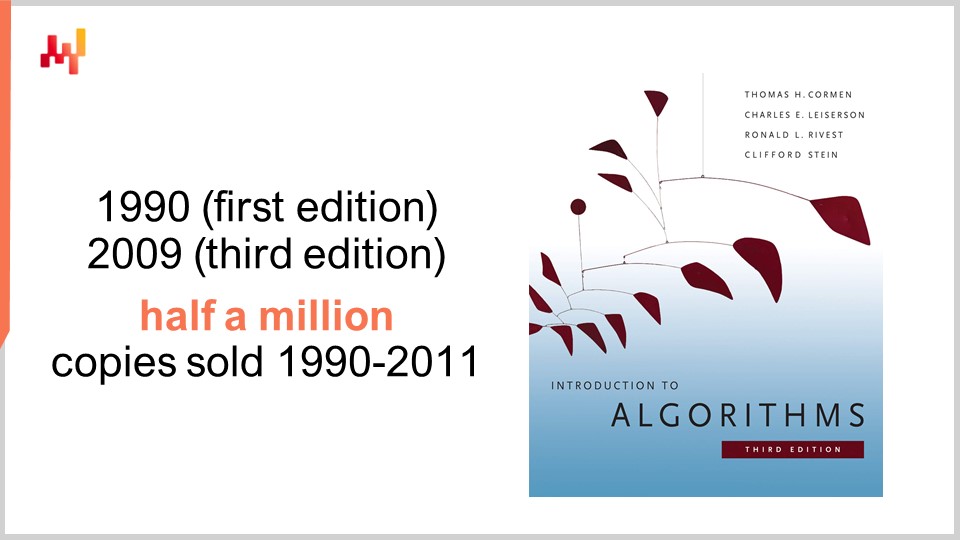
In terms of algorithms, there is one book that is an absolute reference: Introduction to Algorithms, first published in 1990. It is a must-read book. The quality of presentation and writing is simply over the top. This book sold over half a million copies during its first 20 years of life and inspired an entire generation of academic writers. As a matter of fact, most recent supply chain books dealing with supply chain theory that have been published in the last decade have frequently been heavily inspired by the style and presentation found in this book.
Personally, I read this book back in 1997, and it was actually a French translation of the very first edition. It had a profound influence on my entire career. After reading this book, I never saw software the same again. One word of caution, however, is that this book adopts a perspective about the computing hardware that was prevalent at the end of the ’80s and the beginning of the ’90s. As we have seen in the previous lectures in this series, the computing hardware has been progressing rather dramatically over the last couple of decades, and thus some of the assumptions made in this book feel relatively dated. For example, the book assumes that memory accesses have a constant time, no matter how much memory you want to address. This is not the way modern computers work anymore.
Nevertheless, I believe there are certain situations where being simplistic is a reasonable proposition if what you gain in exchange is a much higher degree of clarity and simplicity of exposition. This book does an amazing job on this front. While I advise keeping in mind that some of the key assumptions made throughout the book are dated, it still remains an absolute reference that I would recommend to the entire audience.
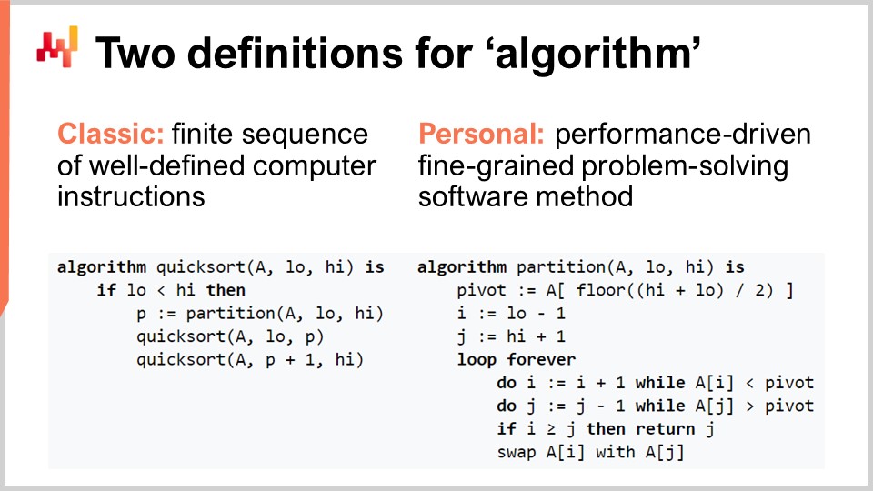
Let’s clarify the term “algorithm” for the audience that might not be that familiar with the notion. There is the classic definition where it’s a finite sequence of well-defined computer instructions. This is the sort of definition you will find in textbooks or on Wikipedia. Although the classic definition of an algorithm has its merits, I believe that it’s underwhelming, as it does not clarify the intent associated with algorithms. It’s not any kind of sequence of instructions that is of interest; it’s a very specific sequence of computer instructions. Thus, I propose a personal definition of the term algorithm: an algorithm is essentially a performance-driven, fine-grained, problem-solving software method.
Let’s unpack this definition, shall we? First, the problem-solving part: an algorithm is completely characterized by the problem it tries to solve. On this screen, what you can see is the pseudocode for the Quicksort algorithm, which is a popular and well-known algorithm. Quicksort tries to solve the sorting problem, which is as follows: you have an array that contains data entries, and you want an algorithm that will return the very same array but with all the entries sorted in increasing order. Algorithms come with a complete focus on a specific and well-defined problem.
The second aspect is how you judge that you have a better algorithm. A better algorithm is something that lets you solve the very same problem with fewer computing resources, which in practice means faster. Finally, there is the fine-grain part. When we say the term “algorithms,” it comes with the idea that we want to look at very elementary problems that are modular and can be composed endlessly to solve much more complicated problems. That’s really what algorithms are about.
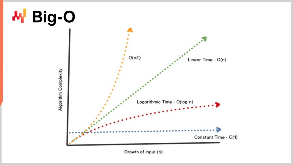
One key achievement of the theory of algorithms is to provide a characterization of the performance of algorithms in a fairly abstract manner. I won’t have the time today to delve into the fine print of this characterization and the mathematical framework. The idea is that, in order to characterize the algorithm, we want to look at the asymptotic behavior. We have a problem that is dependent on one or several key bottleneck dimensions that characterize the problem. For example, in the sorting problem I presented earlier, the characteristic dimension is usually the number of elements to be sorted. The question is, what happens when the array of elements to be sorted becomes very large? I’m going to refer to this characteristic dimension with the number “n” as a convention.
Now, I have this notation, the Big O notation, that you may have seen when dealing with algorithms. I’m just going to outline a few elements to give you an intuition of what’s going on. First, let’s say, for example, we have a dataset, and we want to extract a simple statistical indicator like an average. If I say I have a Big O of 1 algorithm, it means that I am able to return a solution to this problem (computing the average) in constant time, regardless of whether the dataset is small or large. Constant time, or Big O of 1, is an absolute requirement whenever you want to do anything that is real-time in the sense of machine-to-machine communication. If you don’t have something that is constant time, it is very difficult, sometimes impossible, to achieve real-time performance.
Typically, another key performance aspect is Big O of N. Big O of N means that you have a complexity for the algorithm that is strictly linear to the size of the dataset of interest. This is what you get when you have an efficient implementation that is able to solve the problem by just reading the data once or a fixed number of times. Big O of N complexity is typically only compatible with batch execution. If you want to have something that is online and real-time, you can’t have something that goes through the entire dataset, unless you know that your dataset has a fixed size.
Beyond linearity, you have Big O of N squared. Big O of N squared is a very interesting case because it’s the sweet spot of production explosion. It means that the complexity grows quadratically with regard to the size of the dataset, which means that if you have 10 times more data, your performance will be 100 times worse. This is typically the sort of performance where you will not see any problem in the prototype because you’re playing with small datasets. You will not see any problem with the testing phase because, again, you’re playing with small datasets. As soon as you go to production, you have a software that is completely sluggish. Very frequently in the world of enterprise software, especially in the world of supply chain enterprise software, most of the abysmal performance issues that you can observe in the field are actually caused by quadratic algorithms that hadn’t been identified. As a result, you observe the quadratic behavior that is just super slow. This problem was not identified early on because modern computers are quite fast, and N squared is not that bad as long as N is fairly small. However, as soon as you are dealing with a large production-scale dataset, it hurts a lot.

This lecture is actually the second lecture of my fourth chapter in this series of supply chain lectures. In the first chapter, the prologue, I presented my views on supply chain as both a field of study and a practice. What we have seen is that supply chain is a large collection of wicked problems, as opposed to tame problems. Wicked problems cannot be approached by naive methodologies because you have adversarial behaviors all over the place, and thus you need to spend a great deal of attention to the methodology itself. Most naive methods fail in rather spectacular ways. That’s exactly what I’ve done in the second chapter, which is entirely devoted to methodologies that are suitable for studying supply chains and improving the practice of supply chain management. The third chapter, which is not complete yet, is essentially a zoom on what I call “supply chain personnel,” a very specific methodology where we focus on the problems themselves as opposed to the solutions we can think of to address the problem. In the future, I will be alternating between chapter number three and the present chapter, which is about the auxiliary sciences of supply chain.
During the last lecture, we saw that we can get more compute capabilities for our supply chain through better, more modern computing hardware. Today, we are looking at the problem from another angle – we’re looking for more compute capabilities because we have better software. That’s what algorithms are about.
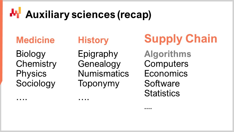
A brief recap: The auxiliary sciences is essentially a perspective on supply chain itself. Today’s lecture is not strictly speaking about supply chain; it is about algorithms. However, I believe it is of foundational importance for supply chain. Supply chain is not an island; the progress that can be achieved in supply chain is very much dependent on the progress that has already been achieved in other adjacent fields. I am referring to those fields as the auxiliary sciences of supply chain.
I believe that the situation is quite similar to the relationship between medical sciences and chemistry during the 19th century. At the very beginning of the 19th century, medical sciences did not care at all about chemistry. Chemistry was still the new kid on the block and not considered a valid proposition for an actual patient. Fast forward to the 21st century, the proposition that you can be an excellent physician while knowing nothing about chemistry would be seen as completely preposterous. It is agreed that being an excellent chemist doesn’t make you an excellent physician, but it is generally agreed upon that if you know nothing about body chemistry, you cannot possibly be competent as far as modern medical sciences are concerned. My take for the future is that during the 21st century, the supply chain field will start to regard the field of algorithms pretty much the same way that the field of medical sciences started to look at chemistry through the 19th century.
Algorithms is a huge field of research, a branch of mathematics, and we will only scratch the surface of this field of research today. In particular, this field of research has been piling up stunning results after stunning results for decades. It may be a fairly theoretical field of research, but it doesn’t mean that it’s just theory. Actually, it is a field of research that is fairly theoretical, but there have been tons of findings that made their way into production.
As a matter of fact, any kind of smartphone or computer that you’re using today is literally using tens of thousands of algorithms that were originally published somewhere. This track record is actually much more impressive compared to the supply chain theory, where the vast majority of supply chains are not running based on the findings of the supply chain theory, not yet. When it comes to modern computers and modern algorithms, virtually everything that is software-related is completely driven by all those decades of findings of algorithmic research. This is very much at the core of virtually every single computer that we are using today.
For the lecture today, I’ve cherry-picked a list of topics that I believe to be quite illustrative of what you should know to approach the topic of modern algorithms. First, we will discuss how we can actually outperform supposedly optimal algorithms, especially for supply chain. Then, we will have a quick look at data structures, followed by magic recipes, tensor compression, and finally, meta techniques.
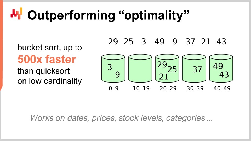
First, I would like to clarify that when I say “algorithms for supply chain,” I don’t mean algorithms that are intended to solve supply chain-specific problems. The correct perspective is to look at classic algorithms for classic problems and revisit those classic problems from a supply chain perspective to see if we can actually do something better. The answer is yes, we can.
For example, the quicksort algorithm, according to the general theory of algorithms, is optimal in the sense that you cannot introduce an algorithm that is arbitrarily better than quicksort. So, in this regard, quicksort is as good as it can ever be. However, if we focus on supply chain specifically, it is possible to achieve stunning speed-ups. In particular, if we look at sorting problems where the cardinality of the datasets of interest is low, such as dates, prices, stock levels, or categories, all of those are low cardinality datasets. Thus, if you have extra assumptions, such as being in a low cardinality situation, then you can use the bucket sort. In production, there are plenty of situations where you can achieve absolutely monumental speed-ups, like 500 times faster than quicksort. So, you can be orders of magnitude faster than what was supposedly optimal just because you’re not in the general case but in the supply chain case. That is something very important, and I believe that here lies the crux of the key stunning results that we can achieve leveraging algorithms for supply chain.
I believe that this perspective is misguided for at least two reasons. First, as we have seen, it is not necessarily the standard algorithm that is of interest. We have seen that there is a supposedly optimal algorithm like quicksort, but if you take the very same problem from a supply chain angle, you can actually achieve massive speed-ups. So, it is of primary interest to be familiar with algorithms, if only to be able to revisit the classics and achieve massive speed-ups just because you are not in the general case but in the supply chain case.
The second reason why I believe that this perspective is misguided is that algorithms are very much about data structures. Data structures are ways you can organize data so that you can operate more efficiently on the data. The interesting thing is that all these data structures form a vocabulary of a kind, and having access to this vocabulary is essential in order to be able to describe supply chain situations in ways that lend themselves to an easy translation into software. If you start with a description using layman terms, then you usually end up with things that are exceedingly hard to translate into software. If you expect a software engineer, who knows nothing about the supply chain, to implement this translation for you, that might be a recipe for trouble. It’s actually much easier if you know this vocabulary, so you can directly speak the terms that lend themselves easily to the translation of the ideas you have into software.
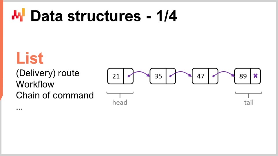
Let’s review the most popular and simplest data structures. The first one would be the list. The list can be used, for example, to represent a delivery route, which would be the sequence of deliveries to be made, with one entry per delivery. You can enumerate the delivery route as you progress through it. A list can also represent a workflow, which is a sequence of operations needed to manufacture a certain piece of equipment, or a chain of command, which determines who is supposed to make certain decisions.
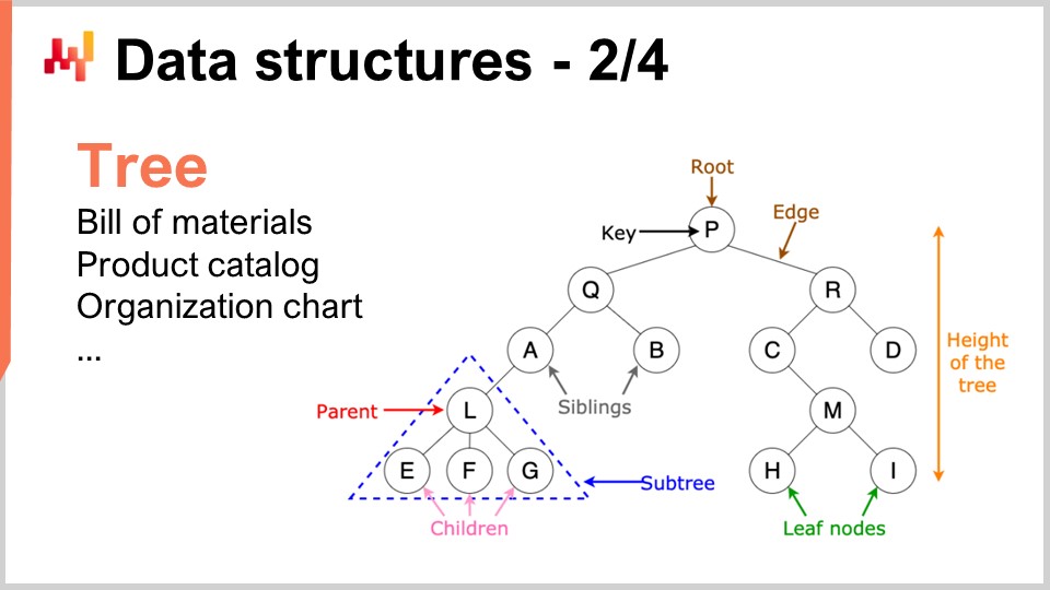
Similarly, trees are another ubiquitous data structure. By the way, algorithmic trees are upside down, with the root at the top and the branches at the bottom. Trees let you describe all kinds of hierarchies, and supply chains have hierarchies all over the place. For example, a bill of material is a tree; you have a piece of equipment that you want to manufacture, and this piece of equipment is made of assemblies. Each assembly is made of sub-assemblies, and each sub-assembly is made of parts. If you expand the bill of material completely, you get a tree. Similarly, a product catalog, where you have product families, product categories, products, subcategories, etc., very frequently has a tree-like architecture attached to it. An organizational chart, with the CEO on top, the C-level executives below, and so on, is also represented by a tree. Algorithmic theory gives you a multitude of tools and methods to process trees and perform operations efficiently over trees. Whenever you can represent data as a tree, you have an entire arsenal of mathematical methods to work efficiently with those trees. That’s why this is of high interest.
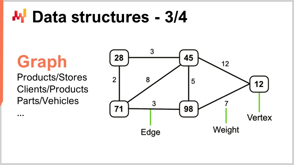
Now, graphs let you describe all sorts of networks. By the way, a graph, in the mathematical sense, is a set of vertices and a set of edges, with edges connecting two vertices together. The term “graph” might be a tiny bit deceptive because it has nothing to do with graphics. A graph is just a mathematical object, not a drawing or anything graphical. When you know how to look for graphs, you will see that supply chains have graphs all over the place.
A few examples: An assortment in a retail network, which is fundamentally a bipartite graph, connects products and stores. If you have a loyalty program where you record which client has bought which product over time, you have yet another bipartite graph connecting clients and products. In the automotive aftermarket, where you have repairs to execute, you typically need to use a compatibility matrix that tells you the list of parts that have mechanical compatibility with the vehicle of interest. This compatibility matrix is essentially a graph. There is an enormous amount of literature on all sorts of algorithms that let you work with graphs, so it’s very interesting when you can characterize a problem as being supported by a graph structure because all the methods known in the literature become readily available.
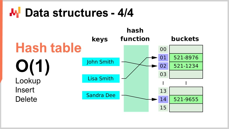
Finally, the last data structure I will be covering today is the hash table. The hash table is essentially the Swiss Army knife of algorithms. It’s not new; none of the data structures I’ve introduced are recent by any standard. The hash table is probably the most recent of the lot, dating from the 1950s, so it’s not recent. Nonetheless, the hash table is an incredibly useful data structure. It’s a container that contains pairs of keys and values. The idea is that with this container, you can store a lot of data, and it gives you big O(1) performance for lookup, insert, and delete. You have a container where you can, in constant time, add data, look whether data is present or not (by looking at the key), and potentially remove data. This is very interesting and useful. Hash tables are literally all over the place and are extensively used inside other algorithms.
One thing I will be pointing out, and we will revisit this point later on, is that the performance of a hash table is very much dependent on the performance of the hash function that you have.
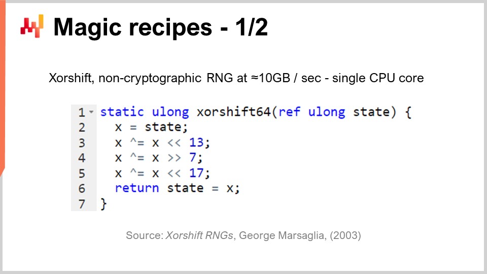
Now, let’s have a look at magical recipes, and we will completely switch to a different perspective. Magical numbers are fundamentally an anti-pattern. In the previous lecture, the one about negative knowledge for supply chain, we discussed how anti-patterns typically start with a good intent but end up with unintended consequences that undo the benefits supposedly brought by the solution. Magic numbers are a well-known programming anti-pattern. This programming anti-pattern consists of writing code littered with constants that seem completely out of the blue, making your software very hard to maintain. When you have tons of constants, it’s unclear why you have those constraints and how they were chosen.
Usually, when you see magic numbers in a program, it’s better to isolate all those constants in a place where they are more manageable. However, there are situations where a careful choice of constants does something completely unexpected, and you have near-magical, completely unintended benefits of using numbers that seem to have fallen from the sky. This is exactly what the very short algorithm I’m presenting here is about.
In supply chain, very frequently, we want to be able to achieve simulation of a kind. Simulations or Monte Carlo processes are one of the basic tricks you can use in a myriad of supply chain situations. However, the performance of your simulation is very much dependent on your capacity to generate random numbers. To generate simulations, there is usually a degree of generated randomness involved, and thus you need an algorithm to generate this randomness. As far as computers are concerned, it’s typically pseudorandomness – it’s not true randomness; it’s just something that looks like random numbers and has the statistical attributes of random numbers but isn’t actually random.
The question becomes, how efficiently can you generate random numbers? It turns out that there is an algorithm called “Shift,” published in 2003 by George Marsaglia, that is quite impressive. This algorithm generates very high-quality random numbers, creating a complete permutation of 2 to the power of 64 minus 1 bits. It’s going to circulate through all the 64-bit combinations, minus one, with zero as a fixed point. It does this with essentially six operations: three binary shifts and three XOR (exclusive or) operations, which are bitwise operations. The shifts are also bitwise operations.
What we see is that there are three magic numbers in the middle of that: 13, 7, and 17. By the way, all those numbers are prime numbers; this is not an accident. It turns out that if you pick those very specific constants, you get an excellent random number generator that happens to be super fast. When I say super fast, I mean that you can literally generate 10 megabytes per second of random numbers. This is absolutely enormous. If we go back to the previous lecture, we can see why this algorithm is also so efficient. Not only do we have only six instructions that directly map to instructions natively supported by the underlying computing hardware, like the processor, but also we don’t have any branch. There is no test, and thus it means that this algorithm, once executed, will max out the pipelining capacity of the processor because there is no branching. We can literally max out the deep pipelining capacity that we have in a modern processor. This is very interesting.
The question is, could we pick any other numbers to make this algorithm work? The answer is no. There are only a few dozen or maybe about a hundred different combinations of numbers that would actually work, and all the others will give you a number generator of very low quality. That’s where it’s magical. You see, this is a recent trend in algorithmic development, to find something completely unexpected where you find some semi-magical constant that gives you completely unintended benefits by mixing very unexpected binary operations of a kind. Random number generation is of critical importance for supply chain.
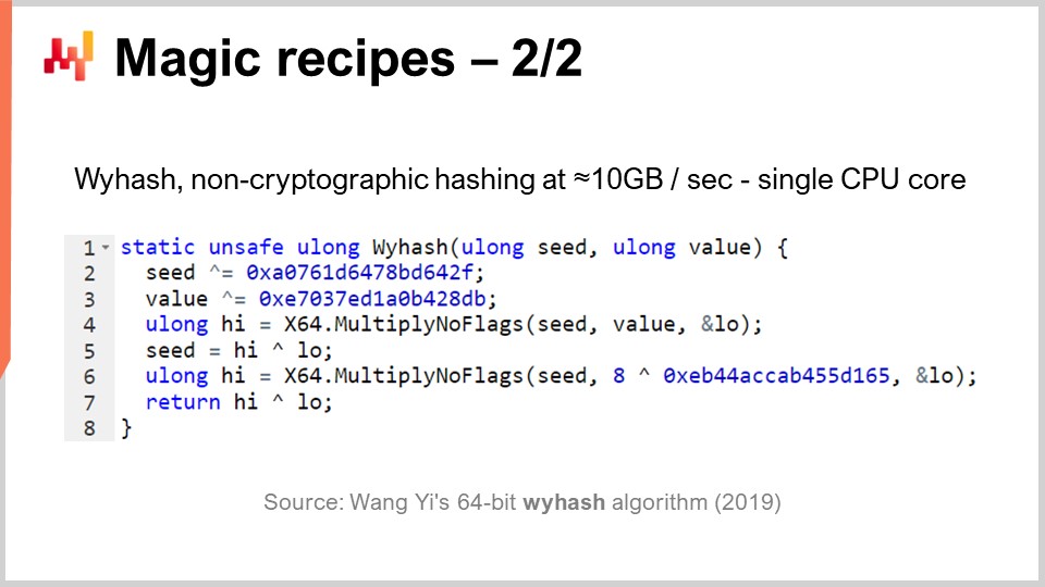
But, as I was saying, hash tables are all over the place, and it’s also of high interest to have a super high-performance generic hash function. Does it exist? Yes. There have been entire classes of hash functions available for decades, but in 2019, another algorithm was published that gives record-breaking performance. This is the one you can see on the screen, “WyHash” by Wang Yi. Essentially, you can see that the structure is very much similar to the XORShift algorithm. It’s an algorithm that has no branch, like XORShift, and it is also using the XOR operation. The algorithm uses six instructions: four XOR operations and two Multiply-No-Flags operations.
Multiply-No-Flags is just the vanilla multiplication between two 64-bit integers, and as a result, you collect the high 64 bits and the low 64 bits. This is an actual instruction available in modern processors, implemented at the hardware level, so it counts as just one computer instruction. We have two of them. Again, we have three magical numbers, written in hexadecimal form. By the way, those are prime numbers, again, completely semi-magical. If you apply this algorithm, you have an absolutely excellent non-cryptographic hash function that is almost operating at the speed of memcpy. It’s very fast and of prime interest.
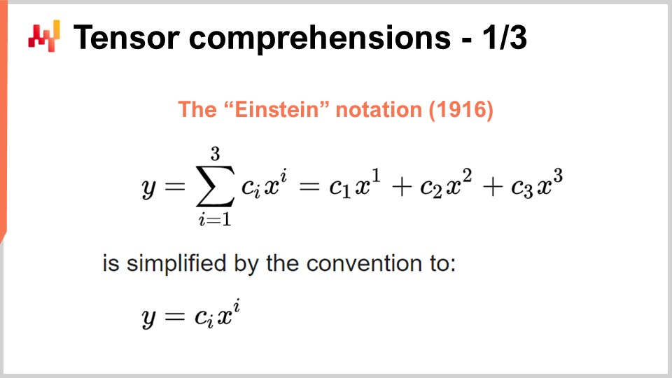
Now, let’s switch to something completely different again. The success of deep learning and many other modern machine learning methods lies in a few key algorithmic insights on the problems that can be massively accelerated by dedicated computing hardware. That’s what I discussed in my previous lecture when I was talking about processors with super-scalar instructions and, if you want more, GPUs and even TPUs. Let’s revisit this insight to see how the whole thing emerged rather chaotically. However, I believe that the relevant insights have crystallized over the last few years. In order to understand where we stand nowadays, we have to go back to the Einstein notation, which was introduced a little over a century ago by Albert Einstein in one of his papers. The intuition is simple: you have an expression y that is a sum from i equal 1 to i equal 3 of c_y times x_y. We have expressions written like that, and the intuition of the Einstein notation is to say, in this sort of situation, we should write it omitting entirely the summation. In software terms, the summation would be a for loop. The idea is to omit the summation entirely and say that by convention, we do the sum on all the indices for the variable i that makes sense.
This simple intuition yields two very surprising but positive outcomes. The first one is design correctness. When we explicitly write the sum, we risk not having the proper indices, which can lead to index-out-of-bounds errors in software. By removing the explicit summation and stating that we will take all the valid index positions by definition, we have a correct-by-design approach. This alone is of primary interest and is related to array programming, a programming paradigm that I briefly touched on in one of my previous lectures.
The second insight, which is more recent and of great interest nowadays, is that if you can write your problem in the form where the Einstein notation applies, your problem can benefit from massive hardware acceleration in practice. This is a game-changing element.
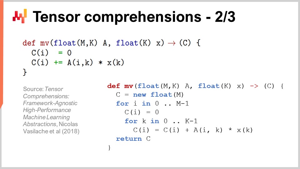
To understand why, there is a very interesting paper called “Tensor Comprehensions” published in 2018 by the Facebook research team. They introduced the notion of tensor comprehensions. First, let me define the two words. In the field of computer science, a tensor is essentially a multi-dimensional matrix (in physics, tensors are completely different). A scalar value is a tensor of dimension zero, a vector is a tensor of dimension one, a matrix is a tensor of dimension two, and you can have tensors with even higher dimensions. Tensors are objects with array-like properties attached to them.
Comprehension is something a bit like an algebra with the four basic operations – plus, minus, multiply, and divide – as well as other operations. It is more extensive than regular arithmetic algebra; that’s why they have a tensor comprehension instead of a tensor algebra. It is more comprehensive but not as expressive as a full-blown programming language. When you have a comprehension, it is more restrictive than a complete programming language where you can do anything you want.
The idea is that if you look at the MV function (def MV), it’s fundamentally a function, and MV stands for matrix-vector. In this case, it is a matrix-vector multiplication, and this function is essentially performing a multiplication between the matrix A and the vector X. We see in this definition that the Einstein notation is at play: we write C_i = A_ik * X_k. What values should we pick for i and k? The answer is all the valid combinations for those variables that are indices. We take all the valid indices values, do the sum, and in practice, this gives us a matrix-vector multiplication.
At the bottom of the screen, you can see the same method MV rewritten with for loops, explicitly specifying the ranges of values. The key achievement of the Facebook research team is that whenever you can write a program with this syntax of tensor comprehension, they have developed a compiler that allows you to benefit extensively from hardware acceleration using GPUs. Basically, they let you accelerate any program that you can write with this tensor comprehension syntax. Whenever you can write a program in this form, you will benefit from massive hardware acceleration, and we are talking about something that is going to be two orders of magnitude faster than a regular processor. This is a stunning result in its own merit.
Now let’s have a look at what we can do from a supply chain perspective with this approach. One key interest for modern supply chain practice is probabilistic forecasting. Probabilistic forecasting, which I addressed in a previous lecture, is the idea that you are not going to have a point forecast, but rather you are going to forecast all the various probabilities for a variable of interest. Let’s consider, for example, a lead time forecast. You want to forecast your lead time and have a probabilistic lead time forecast.
Now let’s say your lead time can be decomposed into the manufacturing lead time and the transport lead time. In reality, you most likely have a probabilistic forecast for the manufacturing lead time, which is going to be a discrete random variable giving you the probability of observing a time of one day, two days, three days, four days, etc. You can think of it as a large histogram that gives you the probabilities of observing this duration for the manufacturing lead time. Then you’re going to have a similar process for the transport lead time, with another discrete random variable providing a probabilistic forecast.
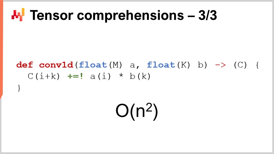
Now you want to calculate the total lead time. If the forecasted lead times were numbers, you would just do a simple addition. However, the two forecasted lead times are not numbers; they are probability distributions. So, we have to combine these two probability distributions to obtain a third probability distribution, which is the probability distribution for the total lead time. It turns out that if we make the assumption that the two lead times, manufacturing lead time and transportation lead time, are independent, the operation we can do to perform this summation of random variables is just a one-dimensional convolution. It may sound complex, but it’s not actually that complex. What I’ve implemented, and what you can see on the screen, is the implementation of a one-dimensional convolution between a vector that represents the histogram for the probabilities of the manufacturing lead time (A) and the histogram associated with the probabilities of the transport lead time (B). The result is the total time, which is the sum of those probabilistic lead times. If you use the tensor comprehension notation, this can be written in a very compact, one-line algorithm.
Now, if we go back to the Big O notation that I introduced earlier in this lecture, we see that we have fundamentally a quadratic algorithm. It is Big O of N^2, with N being the characteristic size of the arrays for A and B. As I mentioned, quadratic performance is a sweet spot of prediction woes. So, what can we do to address this problem? First, we have to consider that this is a supply chain problem, and we have the law of small numbers that we can use to our advantage. As we discussed in the previous lecture, supply chains are predominantly about small numbers. If we’re looking at lead times, we can reasonably assume that those lead times will be smaller than, let’s say, 400 days. That’s already quite a long time for this histogram of probability.
So, what we are left with is a Big O of N^2, but with N smaller than 400. 400 can be quite large, as 400 times 400 is 160,000. That’s a significant number, and remember that adding to this probability distribution is a very basic operation. As soon as we start to do probabilistic forecasting, we will want to combine our forecasts in various ways, and we will most likely end up doing millions of these convolutions, just because fundamentally, these convolutions are nothing but glorified addition projected in the realm of random variables. Thus, even if we have constrained N to be smaller than 400, it is of great interest to bring hardware acceleration to the table, and that’s precisely what we can achieve with tensor comprehension.
The key thing to remember is that as soon as you can write that algorithm, you want to leverage what you know about the supply chain concepts to clarify the applicable assumptions and then leverage the toolkits you have to obtain hardware acceleration.
Now, let’s discuss meta techniques. Meta techniques are of high interest because they can be layered on top of existing algorithms, and thus, if you have an algorithm, there is a chance that you can use one of these meta techniques to improve its performance. The first key insight is compression, simply because smaller data means faster processing. As we have seen in the previous lecture, we don’t have uniform memory access. If you want to access more data, you need to access different types of physical memory, and as memory grows, you get to different types of memory that are much less efficient. The L1 cache inside the processor is very small, around 64 kilobytes, but it is very fast. The RAM, or main memory, is several hundred times slower than this small cache, but you can have literally a terabyte of RAM. Thus, it is of great interest to make sure that your data is as small as possible, as this will almost invariably make your algorithms run faster. There is a series of tricks that you can use in this regard.
First, you can clean up and tidy your data. This is the realm of enterprise software. When you have an algorithm that runs against data, there is often a lot of unused data that does not contribute to the solution of interest. It is essential to ensure that you don’t end up with the data of interest being interleaved with data that happens to be ignored.
The second idea is bit packing. There are plenty of situations where you can pack some flags inside other elements, such as pointers. You might have a 64-bit pointer, but it is very rare that you actually need a 64-bit address range to the full extent. You can sacrifice a few bits of your pointer to inject some flags, which lets you minimize your data with almost no loss of performance whatsoever.
Also, you can tune your precision. Do you need 64 bits of floating-point precision in supply chain? It is very rare that you actually need this precision. Usually, 32 bits of precision is enough, and there are even plenty of situations where 16 bits of precision is sufficient. You might think that reducing precision is not significant, but frequently, when you can divide the size of the data by a factor of two, you don’t merely speed up your algorithm by a factor of 2; you literally speed it up by a factor of 10. Packing the data yields completely nonlinear benefits in terms of speed of execution.
Finally, you have entropy coding, which is essentially compression. However, you don’t necessarily want to use algorithms that are as efficient to compress as, let’s say, the algorithm used for a ZIP archive. You want something that might be a little less efficient in terms of compression but much faster in execution.
Compression fundamentally revolves around the idea that you can trade a bit of extra CPU usage to decrease the pressure on memory, and in almost all situations, this is the trick of interest.
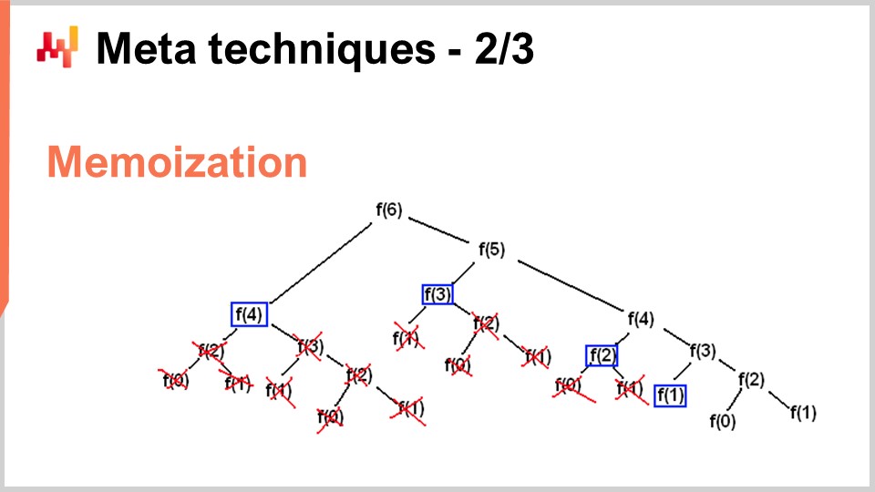
However, there are situations where you want to do the exact opposite – trade memory to vastly reduce your consumption of CPU. That’s precisely what you’re doing with the memoization trick. Memoization is fundamentally the idea that if a function is called many times during the course of the execution of your solution, and the same function is being called with the very same inputs, you don’t need to recompute the function. You can record the result, put it aside (for example, in a hash table), and when you revisit the same function, you will be able to check whether the hash table already contains a key associated with the input or whether the hash table already contains the result because it has been precomputed. If the function you are memoizing is very expensive, you can achieve a massive speed-up. Where it gets very interesting is when you start using memoization not with the main memory, as we have seen in the previous lecture, DRAM is very expensive. It becomes very interesting when you start putting your results on disk or SSDs, which are cheap and plentiful. The idea is that you can trade SSDs in exchange for a reduction of CPU pressure, which is, in a way, the exact opposite of the compression I was just describing.
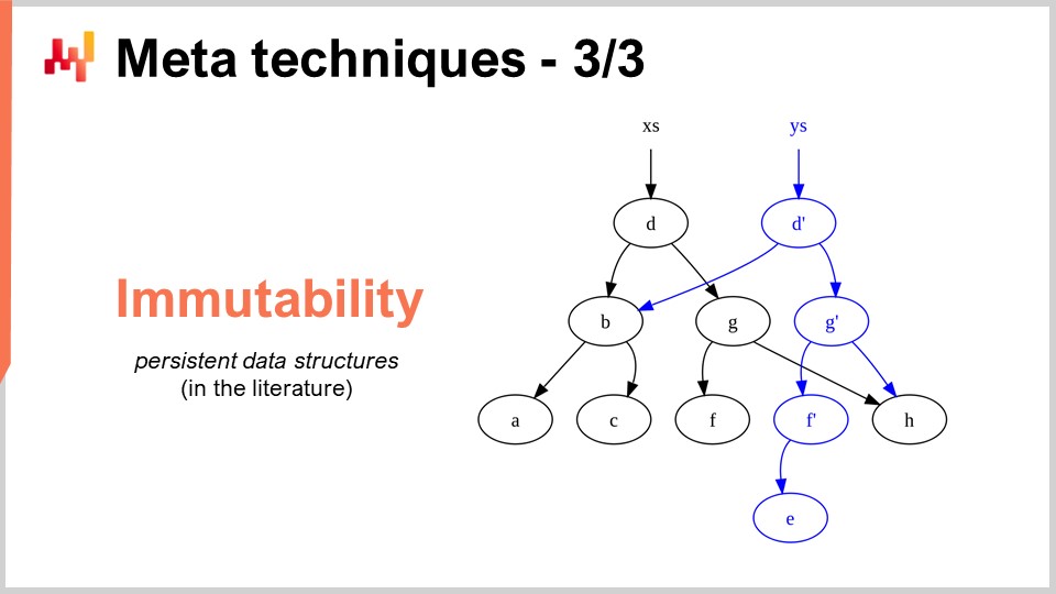
The last meta-technique is immutability. Immutable data structures are fundamentally data structures that are never modified. The idea is that changes get layered on top. For example, with an immutable hash table, when you add an element, what you are going to return is a new hash table that contains everything in the old hash table plus the new element. The very naive way to do that is to do an entire copy of the data structure and return the whole copy; however, it’s very inefficient. The key insight with immutable data structures is that when you modify the data structure, you return a new data structure that only implements the change, but this new data structure recycles all the parts of the old data structure that have not been touched.
Nearly all classic data structures, such as lists, trees, graphs, and hash tables, have their immutable counterparts. In many situations, it is of high interest to use those. By the way, there are modern programming languages that went completely all the way in immutability, like Clojure, for example, for those of you who may be familiar with this programming language.
Why is it of high interest? First, because it massively simplifies the parallelization of algorithms. As we have seen in the previous lecture, it is not possible to find a processor that runs at 100 GHz for general desktop computer processors. What you can find, however, is a machine with 50 cores, each core running at 2 GHz. If you want to take advantage of those many cores, you have to parallelize your execution, and then your parallelization is at risk of very nasty bugs called race conditions. It becomes very difficult to understand whether the algorithm you’ve written is correct or not because you might have various processors that, at the same time, try to write to the same piece of memory in the computer.
However, if you have immutable data structures, this never happens by design, just because once a data structure is presented, it will never change—only a new data structure will emerge. Thus, you can achieve a massive performance speed-up with the immutable path just because you can more easily implement parallel versions of your algorithms. Keep in mind that usually, the bottleneck to implementing algorithmic speed-up is the time it takes to actually implement the algorithms. If you have something that, by design, lets you apply some kind of fearless concurrency principle, you can actually roll out algorithmic speed-ups much faster, with fewer resources in terms of the number of programmers involved. Another important benefit of immutable data structures is that they greatly facilitate debugging. When you modify destructively a data structure and encounter a bug, it might be very difficult to figure out how you got there. With a debugger, it can be quite a nasty experience to pinpoint the problem. The interesting thing with immutable data structures is that changes are non-destructive, so you can see the previous version of your data structure and more easily grasp how you got to the point where you face some kind of incorrect behavior.

To conclude, better algorithms can feel like superpowers. With better algorithms, you get more from the very same computing hardware, and those benefits are indefinite. It’s a one-time effort, and then you have an indefinite upside because you have gained access to superior compute capabilities, considering the same amount of computing resources dedicated to a given supply chain problem of interest. I believe that this perspective offers opportunities for massive improvements in supply chain management.
If we look at a completely different field, such as video games, they have established their own algorithmic traditions and findings dedicated to the gaming experience. The stunning graphics you experience with modern video games are the product of a community that spent decades rethinking the entire algorithm stack to maximize the quality of the gaming experience. The perspective in gaming is not to have a 3D model that is correct from a physical or scientific perspective, but to maximize the perceived quality in terms of the graphic experience for the player, and they have fine-tuned algorithms to achieve stunning results.
I believe that this sort of work has barely started for supply chains. Enterprise supply chain software is stuck, and in my own perception, we are not using even 1% of what modern computing hardware can do for us. Most of the opportunities lie ahead and can be captured through algorithms, not just supply chain algorithms like vehicle routing algorithms, but in revisiting classic algorithms from a supply chain perspective to achieve massive speed-ups along the way.

Now, I will have a look at the questions.
Question: You have been talking about the supply chain specifics, like small numbers. When we know in advance we have small numbers across our potential decisions, what kind of simplification does this bring? For example, when we know we can order one or two containers at most, can you think of any concrete examples of how this would influence the granularity level of holistic forecasts that will be used to compute the stock reward function?
First, everything that I’ve presented today is in production at Lokad. All of these insights, one way or another, are very much applicable to supply chain because they are in production at Lokad. You have to realize that what you get from modern software is something that has not been tuned to make the most of the computing hardware. Just think that, as I presented in my last lecture, we have computers nowadays that are a thousand times more capable than computers we had a few decades ago. Do they run a thousand times faster? They don’t. Can they tackle problems that are fantastically more complicated than what we had a few decades ago? They don’t. So don’t underestimate the fact that there are very large potentials for improvement.
The bucket sort that I have presented in this lecture is a simple example. You have sorting operations all over the place in supply chain, and to my knowledge, it is very rare that you have any enterprise piece of software that takes advantage of specialized algorithms that fit nicely with supply chain situations. Now, when we know that we have one or two containers, do we take advantage of those elements at Lokad? Yes, we do all the time, and there are tons of tricks that can be implemented at that level.
The tricks are usually at a lower level, and the benefits will just bubble up to the overall solution. You have to think about decomposing container filling problems into all their subparts. You can have benefits by applying the ideas and tricks that I’ve presented today at the lower level.
For example, what sort of numerical precision do you need if we are talking about containers? Maybe 16-bit numbers with only 16 bits of precision might suffice. That makes the data smaller. How many distinct products are we ordering? Maybe we are only ordering a few thousand distinct products, so we can use the bucket sort. The probability distribution is a lower, smaller number, so in theory, we have histograms that can go from zero units, one unit, three units, up to infinity, but do we go to infinity? No, we don’t. Maybe we can make some smart assumptions about the fact that it is very rare that we will face a histogram where we exceed 1,000 units. When we have that, we can approximate. We don’t necessarily need to have a 2-unit precision if we are dealing with a container that contains 1,000 units. We can approximate and have a histogram with bigger buckets and these sorts of things. It’s not as much, I would say, about introducing algorithmic principles like tensor comprehension, which are incredible because they simplify everything in a very cool way. However, most of the algorithmic speed-ups in the end result in a faster but slightly more complicated algorithm. It’s not necessarily simpler because usually, the simplest algorithm is also kind of inefficient. A more appropriate algorithm for a case might be a bit longer to write and more complex, but in the end, it will run faster. This is not always the case, as we have seen with the magical recipes, but what I wanted to show was that we need to revisit the fundamental building blocks of what we are doing to actually build enterprise software.
Question: How widely are these insights implemented in ERP vendors, APS, and best of breeds like GTA?
The interesting thing is that these insights are fundamentally, most of them, completely incompatible with transactional software. Most enterprise software is built around a core that is a transactional database, and everything is channeled through the database. This database is not a supply chain-specific database; it’s a generic database that’s supposed to be able to deal with all the possible situations you can think of, from finance to scientific computing, to medical records, and more.
The problem is that if the piece of software you’re looking at has a transactional database at its core, then the insights I have proposed cannot be implemented by design. It’s kind of game over. If you look at video games, how many video games are built on top of a transactional database? The answer is zero. Why? Because you can’t have good graphics performance implemented on top of a transactional database. You can’t do computer graphics in a transactional database.
A transactional database is very nice; it gives you transactionality, but it locks you up in a world where nearly all the algorithmic speed-ups that you could think of just cannot apply. I believe when we start thinking about APS, there’s nothing advanced about these systems. They have been stuck in the past for decades now, and they are stuck because at the core of their design, they are completely designed around a transactional database that prevents them from applying any of the insights that have emerged from the field of algorithms for the last probably four decades.
That’s the crux of the problem in the field of enterprise software. The design decisions you make in the first month of the design of your product will haunt you for decades, essentially until the end of time. You can’t upgrade once you’ve decided on a specific design for your product; you’re stuck with it. Just like you can’t simply re-engineer a car to be an electric car, if you want to have a very good electric car, you will re-engineer the car entirely around the idea that the propulsion engine is going to be electric. It’s not about merely swapping the engine and saying, “Here is an electric car.” It doesn’t work like that. This is one of those core design principles where once you’ve committed to producing an electric car, you need to rethink everything around the engine so that it’s a good fit. Unfortunately, ERPs and APS that are very much database-centric just cannot use any of these insights, I’m afraid. It is always possible to have an isolated bubble where you benefit from these tricks, but it’s going to be a bolted-on add-on; it’s never going to make it to the core.
Regarding the impressive capabilities of Blue Yonder, please bear with me, as Lokad is a direct competitor of Blue Yonder, and it’s challenging for me to be completely unbiased. In the enterprise software market, you have to make ridiculously bold claims to stay competitive. I’m not convinced that there is any substance to any of those claims. I challenge the premise that anybody in this market has anything that would qualify as impressive.
If you want to see something stunning and ultra-impressive, look at the latest demo for the Unreal Engine or specialized video game algorithms. Consider the computer graphics on next-generation PlayStation 5 hardware; it is absolutely stunning. Do we have anything in the same ballpark of technological achievement in the field of enterprise software? As far as Lokad is concerned, I have a super biased opinion, but looking at the market more generally, I see an ocean of people who have been trying to max out relational databases for decades. Sometimes they bring other types of databases, like graph databases, but that completely misses the point of the insights I’ve presented. It doesn’t provide anything of substance to deliver value to the world of supply chain.
The key message here for the audience is that it’s a matter of design. We have to make sure that the initial decisions that went into the design of your enterprise software are not the sort of things that would, by design, prevent these classes of techniques from even being used in the first place.
The next lecture will happen three weeks from now, on Wednesday at 3 p.m. Paris time. It will be June 13th, and we will revisit the third chapter, which is about supply chain personnel, surprising personality traits, and fictitious companies. Next time, we will talk about cheese. See you then!
