00:21 Introduction
01:53 From forecasting to learning
05:32 Machine learning 101
09:51 The story so far
11:49 My predictions for today
13:54 Accurate on data we don’t have 1/4
16:30 Accurate on data we don’t have 2/4
20:03 Accurate on data we don’t have 3/4
25:11 Accurate on data we don’t have 4/4
31:49 Glory to the template matcher
35:36 A deepness in the learning 1/4
39:11 A deepness in the learning 2/4
44:27 A deepness in the learning 3/4
47:29 A deepness in the learning 4/4
51:59 Go big or go home
56:45 Beyond the loss 1/2
01:00:17 Beyond the loss 2/2
01:04:22 Beyond the label
01:10:24 Beyond the observation
01:14:43 Conclusion
01:16:36 Upcoming lecture and audience questions
Description
Forecasts are irreducible in supply chain as every decision (purchasing, producing, stocking, etc.) reflect an anticipation of future events. Statistical learning and machine learning have largely superseded the classic ‘forecasting’ field, both from a theoretical and from a practical perspective. We will attempt to understand what a data-driven anticipation of the future even means from a modern ‘learning’ perspective.
Full transcript
Welcome to the series of supply chain lectures. I’m Joannes Vermorel, and today I will be presenting “Machine Learning for Supply Chain.” We can’t 3D print goods in real-time, and we can’t teleport them to where they should be delivered. Actually, nearly all supply chain decisions need to be taken looking forward, anticipating future demand or price movements, reflecting implicitly or explicitly some anticipated future market conditions either on the demand side or on the supply side. As a result, forecasting is an integral and irreducible part of supply chain. We never know the future for sure; we can only guess about the future with varying degrees of certainty. The goal of this lecture is to understand what machine learning is bringing to the table as far as capturing the future is concerned.
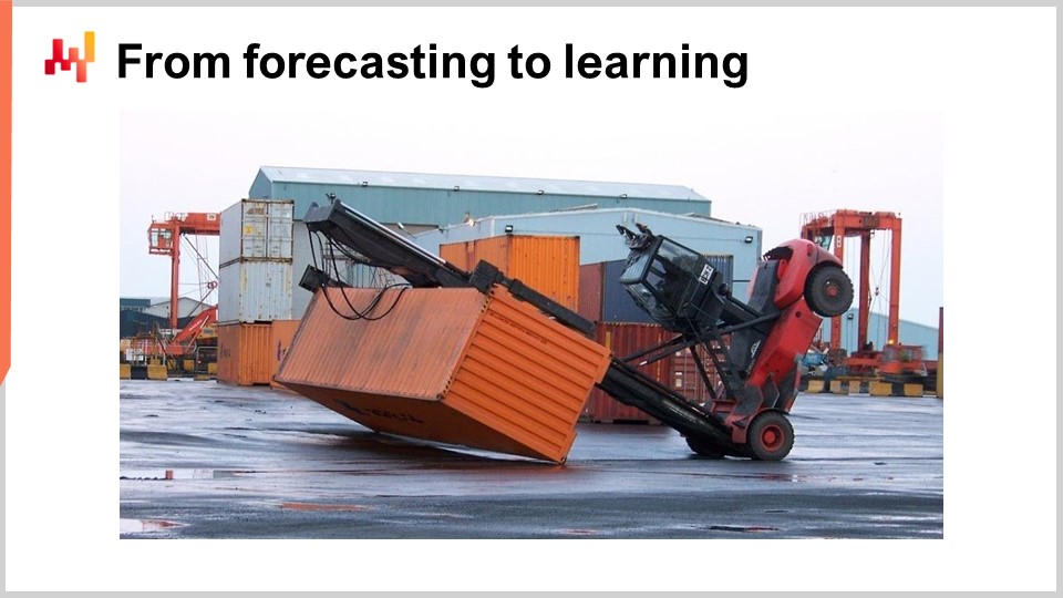
We will see in this lecture that delivering more accurate forecasts is, in the grand scheme of things, a relatively secondary concern. In fact, in supply chain nowadays, forecasting means time series forecasting. Historically, time series forecasts became popular at the beginning of the 20th century in the US. Indeed, the US was the first country to have millions of middle-class employees who were also owning stocks. As people wanted to be savvy investors, they wanted to have insights about their investments, and it turned out that time series and time series forecasts were an intuitive and effective way to convey those insights. You could have time series forecasts about future market prices, future dividends, and future market shares.
In the ‘80s and ‘90s, when supply chain got essentially digitalized, supply chain enterprise software started to benefit from time series forecasts as well. Actually, time series forecasts became ubiquitous in those sorts of enterprise software. However, if you look at this picture, you can realize that time series forecasts are actually a very simplistic and naive way to look at the future.
You see, if I just look at this picture, I can already tell what will happen next: most likely a crew will show up, they will clean up this mess, and very likely they will then inspect the forklifts for safety reasons. They might even perform some light repairs, and with a high degree of confidence, I can say that most likely this forklift will soon be put back in operation. Just looking at this picture, we can also predict what sort of conditions led to this situation. None of this fits the perspective of a time series forecasting, and yet all of these predictions are very relevant.
These predictions are not about the future per se, as this picture was taken a while ago, and even the events that followed this picture being taken are now part of our past. But nonetheless, they are predictions in the sense that we are making statements about things that we don’t know for sure. We don’t have a direct measurement. So the primary thing of interest is, how am I even able to produce these predictions and make these statements?
It turns out that as a human being, I’ve lived, I’ve witnessed events, and I’ve learned from them. That’s how I can actually produce these statements. And it turns out that machine learning is just that: it is the ambition of being able to replicate this capacity for learning with machines, the preferred sort of machines by far being computers nowadays. At this point, you might be wondering how machine learning is even different from other terms like artificial intelligence, cognitive technologies, or statistical learning. Well, it turns out that these terms say a lot more about the people who use them rather than about the problem itself. Problem-wise, the boundaries between all those fields are very fuzzy.
Now let’s dig in with a review of the archetype of machine learning frameworks, covering a short series of central machine learning concepts. Most scientific papers and software produced in this field of machine learning are leveraging this framework to a fairly large extent. The feature represents a piece of data that is made available in order to perform the prediction task. The idea is that you have a prediction task you want to perform, and a feature (or several features) represents what is made available to perform that task. In the context of time series forecasts, the feature would represent the past section of the time series, and you would have a vector of features representing all the past data points.
The label represents the answer to the prediction task. In the case of a time series forecast, it typically represents the portion of the time series that you don’t know, where the future lies. If you have a set of features plus a label, it is referred to as an observation. The typical machine learning setup assumes that you have a dataset containing both features and labels, which represents your training data set.
The goal is to create a program called the model that takes the features as input and computes the desired predicted label. This model is typically engineered through a learning process that goes through the entire training dataset and builds the model. The learning in machine learning is the part where you actually construct the program that makes the predictions.
Finally, there is the loss. The loss is essentially the difference between the real label and the predicted one. The goal is for the learning process to generate a model that makes predictions that are as close as possible to the true labels. You want a model that keeps the predicted labels as close as possible to the true labels.
Machine learning can be seen as a vast generalization of time series forecasting. From the machine learning perspective, features can be anything, not just a past segment of a time series. Labels can also be anything, not just the future segment of a time series. The model can be anything, and even the loss can be pretty much anything. So, we have a framework that is vastly more expressive than time series forecasts. However, as we will see, most of the main achievements of machine learning as a field of study and practice stem from the discoveries of elements that force us to revisit and challenge the list of concepts that I have just briefly introduced.

This lecture is the fourth lecture in the series of supply chain lectures. Auxiliary sciences represent elements that are not supply chain per se but represent something of foundational importance for supply chain. In the first chapter, I presented my views about supply chain both as a physical study and as a practice. In the second chapter, we reviewed a series of methodologies required to tackle a domain like supply chain that presents many adversarial behaviors and cannot be easily isolated. The third chapter is entirely dedicated to supply chain personas, which is a way to focus on the problems we are trying to solve.
In this fourth chapter, I have been gradually going through the ladder of abstraction, starting with computers, then algorithms, and the previous lecture on mathematical optimization, which can be seen as the base layer of modern machine learning. Today, we are venturing into machine learning, which is essential for capturing the future that is prevalent in all the supply chain decisions we need to take every single day.
So, what’s the plan for this lecture? Machine learning is an enormous field of research, and this lecture will be guided by a short series of questions that relate to the concepts and ideas I have introduced earlier. We will see how the answers to these questions force us to revisit the very notion of learning and how we approach the data. One of the most spectacular achievements of machine learning is that it has forced us to realize that there is so much more at play compared to the grand initial ambitions of researchers who thought we would be able to replicate human intelligence within a decade.
In particular, we will have a look at deep learning, which is probably the best candidate we have to emulate a higher degree of intelligence at this point in time. Although deep learning has emerged as an incredibly empirical practice, the progress and achievements accomplished through deep learning shed new light on the fundamental perspective of learning from observed phenomena.
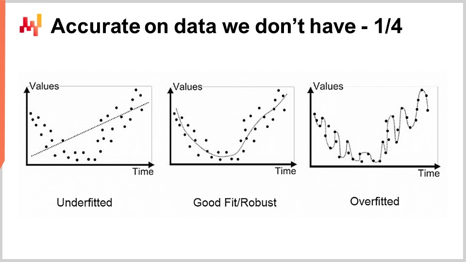
The first problem we have with modeling, statistical or otherwise, is the accuracy of data we don’t have. From a supply chain perspective, this is essential because our interest lies in being able to capture the future. By definition, the future represents a set of data that we don’t have yet. There are techniques, such as backtesting or cross-validation, that can give us some empirical measurements about what we should expect from the accuracy of data that we don’t have. However, why these methods work at all is a relatively intriguing and difficult problem. The problem is not to have a model that fits the data we have; it is easy to build a model that fits the data by using a polynomial with a sufficient degree. Yet, this model is not very satisfying because it is not capturing what we would like to capture.
The classical approach to this problem is known as the bias-variance tradeoff. On the right, we have a model with very few parameters that underfits the problem, which we say has a lot of bias. On the left, we have a model with too many parameters that overfits and has too much variance. In the middle, we have a model that strikes a good balance between bias and variance, which we call a good fit. Until the very end of the 20th century, it was rather unclear how to approach this problem beyond the bias-variance tradeoff.
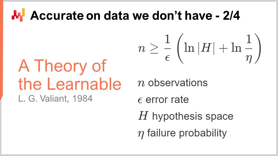
The first true insight about the accuracy of data that we don’t have came from the theories of learnability published by Valiant in 1984. Valiant introduced the PAC theory - Probably Approximately Correct. In this PAC theory, the “probably” part refers to a model with a given probability of giving good enough answers. The “approximately” part means that the answer is not too far from what is considered good or valid.
Valiant showed that in many situations, it is just not possible to learn anything or more precisely that in order to learn, we would need a number of samples that would be so extravagantly large that it would not be practical. This was already a very interesting result. The formula displayed comes from the PAC theory, and it’s an inequality that tells you that if you want to produce a model that is probably approximately correct, you need to have a number of observations, n, greater than a certain quantity. This quantity depends on two factors: epsilon, the error rate (the approximately correct part), and eta, the probability of failing (one minus eta is the probability of not failing).
What we see is that if we want to have a smaller probability of failure or a smaller epsilon (a good enough range), we need more samples. This formula also depends on the cardinality of the hypothesis space. The idea is that the more numerous the competitive hypotheses, the more observations we need to sort them out. This is very interesting because, essentially, although the PAC theory gives us mostly negative results, it tells us what we cannot do, which is to build a provably Probably Approximately Correct model with fewer samples. The theory doesn’t really tell us how to do anything; it’s not very prescriptive in the way to actually become better at solving any kind of prediction task. Nonetheless, it was a landmark because it crystallized the idea that it was possible to approach this problem of accuracy and data that we didn’t have in ways that were much more robust than just doing some very empirical measurements with, let’s say, cross-validation or backtesting.
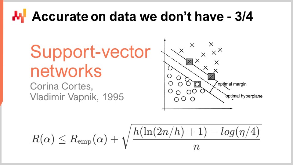
A decade later, the first operational breakthrough came when Vapnik and a few others established what is known today as the Vapnik-Chervonenkis (VC) theory. This theory shows that it’s possible to capture the real loss, referred to as the risk, which is the loss that you will observe on the data that you didn’t have. It was possible to mathematically prove that you had a capacity to know anything about the real error, which, by definition, you cannot ever measure. This is a very puzzling result.
Essentially, this formula, straight out of the VC theory, tells us that the real risk is upper bounded by the empirical risk, which is the risk we can measure on the data that we do have, plus another term frequently referred to as the structural risk. We have the number of observations, n, and eta, which is the probability of failure, just like in the PAC theory. We also have h, which is a measurement of the VC dimension of the model. The VC dimension reflects the capacity of the model to learn; the greater the capacity of the model to learn, the greater the VC dimension.
With these results, we see that for models that have the capacity to learn anything, we cannot say anything about them. This is very puzzling. If your model can learn anything, then you cannot say anything, at least mathematically, about it.
The breakthrough in 1995 came from an implementation by Cortes and Vapnik of what would later be known as Support Vector Machines (SVM). These SVMs are literally the direct implementation of this mathematical theory. The insight is that because we have a theory that gives us this inequality, we can implement a model that balances the amount of error we make on the data (the empirical risk) and the VC dimension. We can directly build a mathematical model that exactly balances these two factors to make the equality as tight as possible and as low as possible. That’s exactly what Support Vector Machines (SVMs) are about. These results were so stunning, operationally, that they gained very good results and had a significant impact on the machine learning community. For the first time, the accuracy on the data that we don’t have wasn’t an afterthought; it was directly obtained by the very mathematical design of the method itself. This was so stunning and powerful that it kept the entire machine learning community distracted for a decade pursuing this path. As we will see, this path turned out to be mostly a dead end, but there was good reason for it: it was an absolutely stunning result.
Operationally, due to the fact that SVMs mostly emerged from a mathematical theory, they had very little mechanical sympathy. They were not a good fit for the computing hardware that we have. More specifically, the naive implementation of SVMs comes with a quadratic cost in terms of memory footprint with regard to the number of observations. This is a lot, and as a consequence, it makes SVMs very slow. There have been later improvements with some online variants of SVMs that have vastly lowered the memory requirements, but nevertheless, SVMs were never really considered as a truly scalable approach to perform machine learning.
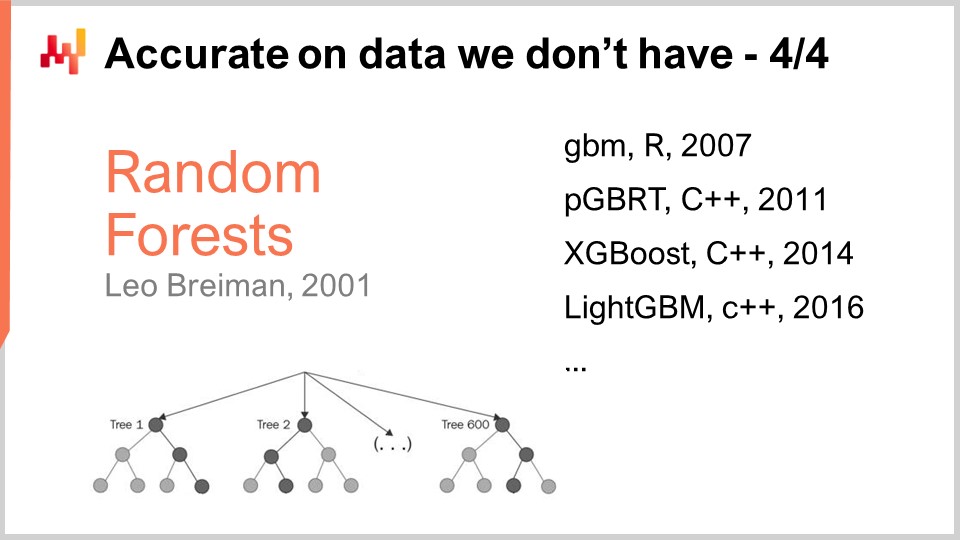
SVMs paved the way for another, better class of models that also probably didn’t overfit. Overfitting is basically being very inaccurate on the data that you don’t have. The most notable examples are probably Random Forests and Gradient Boosted Trees, which happen to be their almost immediate descendants. At their core is boosting, a meta-algorithm that transforms weak models into stronger ones. Boosting emerged from questions raised at the very end of the 80s between Kearns and Valiant, who we mentioned previously in this lecture.
To understand how a Random Forest works, it’s relatively straightforward: take your training dataset and then take a sample of your dataset. On this sample, build a decision tree. Rinse and repeat, creating another sample from the initial training dataset and building another decision tree. Iterate this process, and at the end, you have many decision trees. Decision trees are relatively weak in terms of machine learning models, as they can’t capture very complex patterns. However, if you put all these trees together and average out the results, what you get is a forest, referred to as a Random Forest, because each tree has been built on a randomized subsample of the initial training dataset. What you get with a Random Forest is a much stronger, better machine learning model.
Gradient Boosted Trees are just a minor variation on this insight. The main variation is that, instead of sampling your training dataset and building a tree at random, with all trees being built independently, Gradient Boosted Trees first build the forest, and then the next tree is built by looking at the residuals of the forest that you already have. The idea is that you’ve started to build a model composed of many trees, and you make predictions which diverge from reality. You have these deltas, which are the differences between the real and predicted values, called residuals. The idea is that you’re going to train the next tree not against the original dataset but against a sample of residuals. Gradient Boosted Trees work even better than Random Forests. In practice, Random Forests do overfit, but just a little bit. There are some proofs that show, under certain conditions, Random Forests are not supposed to overfit.
Interestingly, Gradient Boosted Trees have been dominating the high scores of nearly all machine learning competitions for a decade and a half. When you look at about 80-90% of Kaggle competitions, you will see that it’s essentially a Gradient Boosted Tree that landed first. However, despite this incredible dominance in machine learning competitions, there has been very little breakthrough in applying Gradient Boosted Trees to supply chain problems in the wild. The main reason is that Gradient Boosted Trees come with very little mechanical sympathy; their design is not friendly at all to the computing hardware that we have.
It’s straightforward to understand why: you build a model with a series of trees, and the model ends up being as large as a fraction of your dataset. In many situations, you end up with a model that is larger, data-wise, than the dataset you started with. So, if your dataset is already very large, then your model is gigantic, and that is a very problematic issue.
In terms of the history of Gradient Boosted Trees, there has been a series of implementations, starting with GBM (Gradient Boosted Machines) in 2007, which really popularized this approach in an R package. From the very beginning, there were problems with scalability. People quickly started to parallelize the execution with PGBRT (Parallel Gradient Boosted Regression Trees), but it was still very slow. XGBoost was a landmark because it gained an order of magnitude in scalability. The key insight in XGBoost was to adopt a columnar design in the data to make the tree construction faster. Later on, LightGBM recycled all the insights of XGBoost but changed the strategy on how to build the trees. XGBoost grew the tree level-wise, while LightGBM decided to grow the tree leaf-wise. The net result is that LightGBM is now several orders of magnitude faster, considering the same computing hardware, than GBM ever was. Yet, from a practical supply chain perspective, using Gradient Boosted Trees is usually impractically slow. It’s not impossible to use them; it’s just that it’s such a hurdle that it’s usually not worth it.

The puzzling thing is that Gradient Boosted Trees are powerful enough to win nearly all machine learning competitions, and yet, in my humble opinion, these models are a technological dead-end. Support Vector Machines, Random Forests, and Gradient Boosted Trees all have in common that they are nothing more than template matches. They are very good template matches, mind you, but really nothing more. What they are doing exceedingly well is essentially variable selection, and they are very good at that, but there is very little to it. In particular, there is no expressiveness in their capacity to transform the input into anything other than a direct selection or filtering of the input.
If we go back to the forklift image I presented at the very beginning of this lecture, there is no hope whatsoever that any of those models could make the same sort of statements I just made, no matter how large the dataset of images. You could literally feed all those models with millions of images taken from warehouses worldwide, and they still wouldn’t be able to make statements like, “Oh, I’ve seen a forklift in this situation; a crew will show up and do repairs.” Not really.
In practice, what we have seen is that the fact that these models are winning machine learning competitions is deceptive because there are factors that play in their favor in such situations. First, real-world datasets are very complex, which is different from machine learning competitions where, at best, you have toy datasets representing only a fraction of the complexities faced in real-world setups. Second, in order to win a machine learning competition using models like Gradient Boosted Trees, you have to do extensive feature engineering. Due to the fact that these models are glorified template matches, you need to have the right features so that just the selection of variables makes the model work great. You have to inject a high dose of human intelligence into the data preparation for it to work. This is a big problem because, in the real world, when trying to solve a problem for real supply chains, the number of engineering hours you can spend on the problem is limited. You can’t spend six months on a tiny, limited-time, toy problem aspect of your supply chain.
The third issue is that, in supply chains, datasets are constantly changing. It’s not only that the data changes, but the problem is also gradually changing. This compounds the problems you have with feature engineering. Fundamentally, we are left with models that win machine learning and forecasting competitions, but if we start to look a decade ahead, we see that these models are not the future of machine learning; they’re the past.
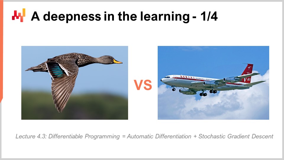
Deep learning was the response to these shallow template matches. Deep learning is often presented as the descendant of artificial neural networks, but the reality is that deep learning only took off the day researchers decided to give up on biological metaphors and focus instead on mechanical sympathy. Again, mechanical sympathy, which means playing nice with the computers we have, is essential. The problem we had with artificial neural networks is that we were trying to mimic biology, but the computers we have are completely unlike the biological substrates that support our brains. This situation is reminiscent of early aviation history, where numerous inventors tried to build flying machines by imitating birds. Nowadays, we have flying machines that fly many times faster than the fastest birds, but the way these machines fly has almost nothing in common with how birds fly.
The first insight about deep learning was the need for something deep and expressive that could apply any kind of transformation to the input data, allowing smart predictive behavior to emerge from the model. However, it also needed to play nice with the computing hardware we had. The idea was that if we had complex models that played very nice with the computing hardware, we would most likely be able to learn functions that are several orders of magnitude more complex, all things considered equal, compared to any method that would not have the same degree of mechanical sympathy.
Differentiable programming, which was presented in the previous lecture, can be considered as the base layer of deep learning. I’m not going to go back to differentiable programming in this lecture, but I invite the audience to watch the previous lecture if you have not seen it. You should be able to understand what follows even if you haven’t seen the previous lecture. The previous lecture should clarify some of the nitty-gritty details of the learning process itself. In summary, differentiable programming is just a way to, if we choose a specific form of model, identify the best values for the parameters that exist within this model.
While differentiable programming focuses on identifying the best parameters, machine learning focuses on identifying the superior forms of models that have the highest capacity to learn from data.
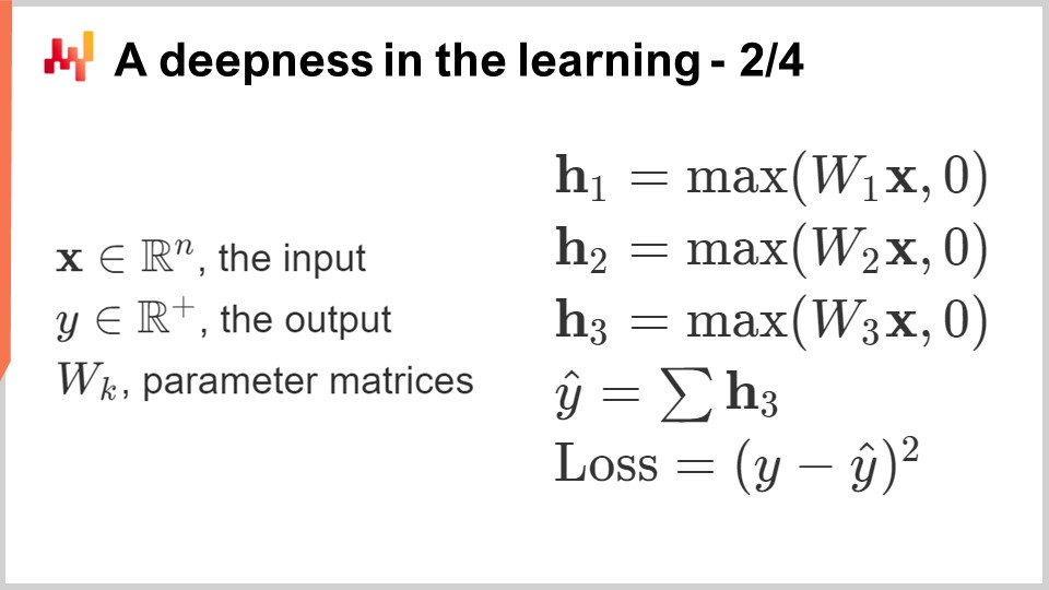
So, how do we create a template for an arbitrarily complex function that can reflect any arbitrarily complex transformation on the input data? Let’s start with a circuit of floating-point values. Why floating-point values? Well, it’s because it’s the sort of thing where we can apply gradient descent, which, as we’ve seen in the previous lecture, is very scalable. So, floating-point numbers it is. We are going to have a sequence of floating-point numbers, which means floating points as inputs and floating points as outputs.
Now, what do we do in the middle? Let’s do linear algebra, and more specifically, let’s do matrix multiplication. Why is that? The answer to why matrix multiplication was given in the very first lecture of this fourth chapter. It relates to the way modern computers are engineered; essentially, it is possible to bring relatively dramatic speed-up in terms of processing speed if you just stick to linear algebra. So, linear algebra it is. Now, if I take my inputs and apply a linear transformation, which is just a matrix multiplication with a matrix named W (this matrix contains the parameters that we want to learn later on), how can we make it more complex? We can add a second matrix multiplication. However, if you remember your linear algebra courses, when you multiply a linear function with another linear function, what you get is a linear function. So, if we just compose the matrix multiplication, we still have a matrix multiplication, and it is still completely linear.
What we are going to do is interleave non-linearities in between the linear operations. This is exactly what I’ve done on this screen. I have interleaved a function typically known in the deep learning literature as a Rectified Linear Unit (ReLU). This name, which is fantastically complicated compared to what it does, is just a very simple function that says if I take a number and if this number is positive, then I return the exact same number (so it’s an identity function), but if the number is negative, I return 0. You can also write it as the max of your value and zero. This is a very trivial non-linearity.
We could use much more sophisticated non-linear functions. Historically, when people were doing neural networks, they wanted to use sophisticated sigmoid functions because that was supposed to be the way it was working in our neurons. But the reality is, why would we want to waste processing power to compute things that are irrelevant? The key insight is that we need to introduce something that is non-linear, and it doesn’t really matter which non-linear function we use. The only thing that matters is to make it very fast. We want to keep the whole thing as fast as possible.
What I’m building here is called dense layers. A dense layer is essentially a matrix multiplication with a non-linearity (the Rectified Linear Unit). We can stack them. On the screen, you can see a network, which is typically called a multi-layer perceptron, and we have three layers. We could keep stacking them, and we could have 20 or 2,000 of them; it doesn’t really matter. The reality is that, as simplistic as it might seem, if you take such a network with just a couple of layers and put it into your differentiable programming framework, which will give you the parameters, the differentiable programming as a base layer will be able to train the parameters, which are initially picked randomly. If you want to initialize it, just initialize all the parameters randomly. You will get fairly decent results for a very large variety of problems.
That is very interesting because, at this point, you have pretty much all the fundamental ingredients of deep learning. So, for the audience, congratulations! You can probably start adding “deep learning specialist” to your resume because this is almost all there is to it. Well, not really, but let’s say it’s a good starting point.
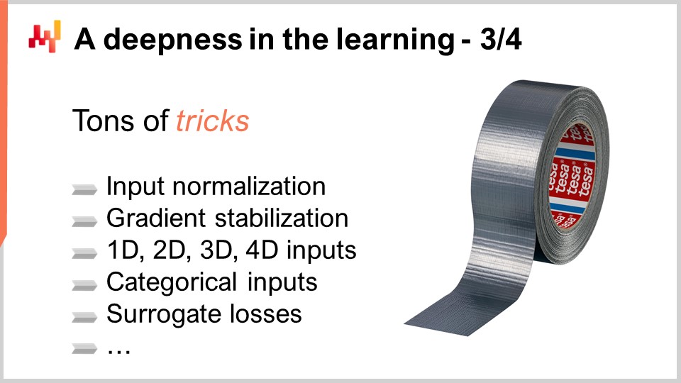
The reality is that deep learning involves very little theory besides tensor algebra, which is essentially computerized linear algebra. However, deep learning involves tons of tricks. For example, we have to normalize the inputs, and we have to stabilize the gradients. If we start stacking many operations like that, the gradients can grow exponentially as we go backward in the network, and at some point, that will overflow the capacity to represent those numbers. We have real-world computers, and they are not able to represent arbitrarily large numbers. At some point, you just overflow your capacity to represent the number with a 32-bit or 16-bit floating-point value. There are tons of tricks for gradient stabilization. For example, the trick is typically batch normalization, but there are other tricks for that.
If you have inputs that have a geometric structure, for example, one-dimensional like a time series (historical sales, as we see in supply chain), that can be two-dimensional (think of it as an image), three-dimensional (that could be a movie), or four-dimensional, etc. If the inputs have a geometric structure, then there are special layers that can capture this geometric structure. The most famous ones are probably called convolutional layers.
Then, you also have techniques and tricks to deal with categorical inputs. In deep learning, all your inputs are floating-point values, so how do you deal with categorical variables? The answer is embeddings. You have surrogate losses, which are alternative losses that exhibit very steep gradients and facilitate the convergence process, ultimately amplifying what you can learn from the data. There are tons of tricks, and all those tricks can typically be thrown into the program you’re composing because we operate with differentiable programming as our base layer.
Deep learning is really about how we compose a program that, once it is run through the training process offered by differentiable programming, has a very high capacity to learn. Most of the items that I’ve just listed on the screen are also of a programmatic nature, which is very convenient considering that we have differentiable programming, a programming paradigm, to support all of that.
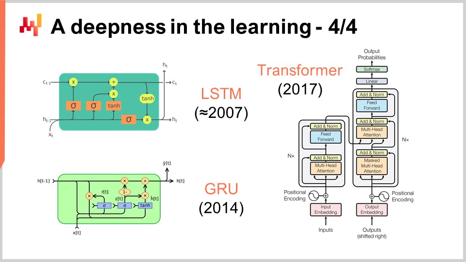
At this point, it should become clearer why deep learning is unlike classic machine learning. Deep learning is not about models. As a matter of fact, most open-source deep learning libraries don’t even include any models. With deep learning, what truly matters are model architectures, which you can think of as templates that need to be heavily customized when you want to fit a specific situation. However, if you adopt a proper architecture, you can anticipate that your customization will still preserve the essence of the capacity of your model to learn. With deep learning, we displace the interest from the final model, which becomes something not very interesting, toward the architecture, which becomes the true matter of research.
On the screen, you can see a series of notable architecture examples. First, LSTM, which stands for Long Short-Term Memory, started working around 2007. The publication history of LSTM is a bit more complicated, but it essentially started working deep learning style in 2007. It was superseded by Gated Recurrent Units (GRU), which is essentially the same thing as LSTM but just simpler and nicer. Essentially, a lot of the LSTM complexity stems from the biological metaphors. It turns out that you can ditch the biological metaphors, and what you get is something simpler that works pretty much the same. That’s Gated Recurrent Units (GRU). Later on, transformers came along, which basically made both LSTM and GRU obsolete. Transformers were a breakthrough as they were much faster, leaner in terms of computing resources needed, and had an even greater capacity to learn.
Most of these architectures come with metaphors. LSTM has a cognitive metaphor, long short-term memory, while transformers come with an information retrieval metaphor. However, these metaphors have very little predictive power, and they might actually be more of a source of confusion and distraction from what really makes these architectures work, which is not entirely well understood at this point.
Transformers are of high interest for supply chain because they are one of the most versatile architectures. They are used for virtually everything nowadays, from autonomous driving to automated translation and many other hard problems. This is a testament to the power of choosing the right architecture, which can then be used to fit a huge diversity of problems. As far as supply chain is concerned, one of the main difficulties of doing anything with machine learning is that we have such an incredible diversity of problems to tackle. We can’t afford to have a team that spends five years on research efforts for every single sub-problem we face. We need something where we can move fast and not have to reinvent half of machine learning whenever we want to solve the next problem.
One aspect of deep learning that is really shocking when you start to think about it is the massive number of parameters. In the multi-layer perceptron I introduced a few minutes ago, with dense layers that involve matrix multiplication, we can have a lot of parameters in those matrices. In fact, it’s not very difficult to have as many parameters as we have data points or observations in our training datasets. As we have seen at the very beginning of our lecture, if we have a model with so many parameters, it should suffer dramatically from overfitting.
The reality with deep learning is even more puzzling. There are many situations where we have vastly more parameters than we have observations, and yet we don’t experience dramatic overfitting problems. Even more puzzling, deep learning models tend to completely fit the training dataset, so you end up having a near-zero error on your training dataset, and they will still retain their predictive power for data that we don’t have.
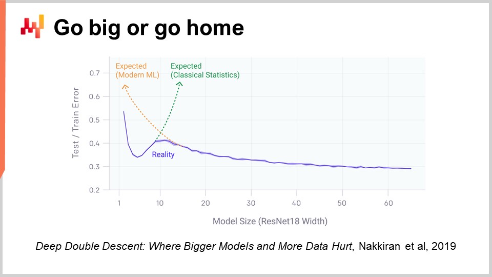
Two years ago, the Deep Double Descent paper published by OpenAI shed some very interesting light on this situation. The team showed that we have essentially an uncanny valley in the realm of machine learning. The idea is that if you take a model and have just a few parameters, you have a lot of bias, and the quality of your results on unseen data is not that good. This conforms to the classic machine learning vision and the classic statistical vision as well. If you increase the number of parameters, you are going to improve the quality of your model, but at some point, you are going to start overfitting. This is exactly what we have seen with the earlier discussion on underfitting and overfitting. There is a balance to be found.
However, what they have shown is that if you keep increasing the number of parameters, something very strange will happen: you are going to overfit less and less, which is the exact opposite of what the classic statistical learning theory would predict. This behavior is not accidental. The authors showed that this behavior is very robust and widespread. It happens pretty much all the time in a large variety of situations. It’s not very well understood yet why, but what is very well understood at this point is that the deep double descent is very real and widespread.
This also helps to understand why deep learning was relatively late to the machine learning party. For deep learning to succeed, we first had to succeed at building models that could process tens of thousands or even hundreds of thousands of parameters to go beyond this uncanny valley. In the 80s and 90s, it would not have been possible to have any deep learning breakthrough, just because the hardware computing resources were not able to jump through this uncanny valley.
Fortunately, with present-day computing hardware, it is possible to train models without much effort that have millions or even billions of parameters. As we pointed out in the previous lectures, there are now companies like Facebook who are training models that have over a trillion parameters. So we can go very far.
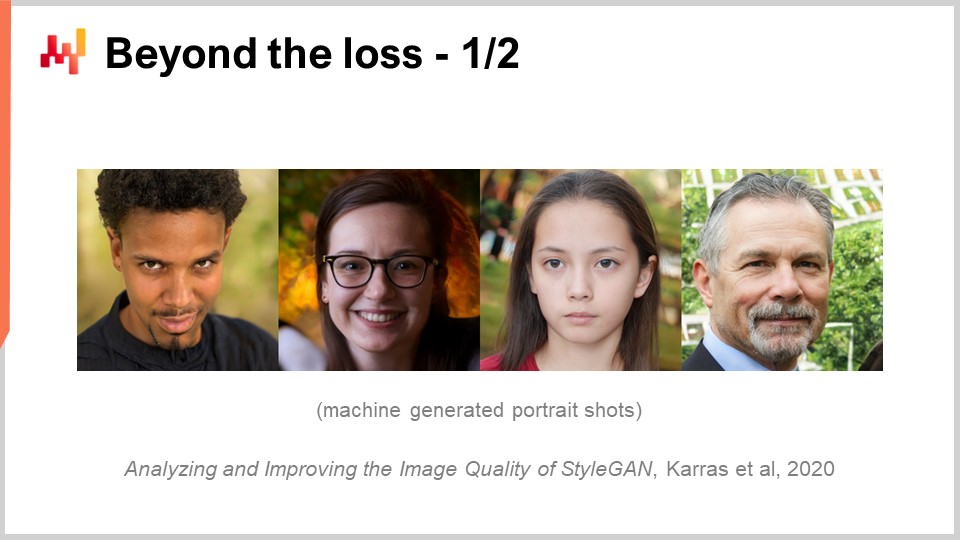
So far, we have assumed that the loss function was known. However, why should it be the case? Indeed, let’s consider the situation of a fashion store from a supply chain perspective. A fashion store has stock levels for every single SKU, and we want to project future demand. We want to project one possible scenario that is believable for future demand for this one store. What will happen is that as certain SKUs run out of stock, we should observe cannibalization and substitution. As a given SKU hits a stockout, normally the demand should, in part, bounce back to similar products.
But if we try to tackle this sort of approach with classic forecasting metrics like Mean Absolute Percentage Error (MAPE), Mean Absolute Error (MAE), Mean Square Error (MSE), or other metrics that operate SKU by SKU, day by day or week by week, we are not going to capture any of these behaviors. What we truly want is a metric that would capture whether we are very good at capturing all those cannibalization and substitution effects. But what should this loss function look like? It’s very unclear, and it seems to require fairly sophisticated behavior. One of the key breakthroughs of deep learning was essentially to come up with the insight that the loss function should be learned. That’s exactly how the image on the screen was produced. This is a fully machine-generated picture; none of those people are real. They have been generated, and the problem was: how do you build a loss function or a metric that tells you whether an image is a good, photorealistic portrait of a human or not?
The reality is that if you start thinking in terms of Mean Absolute Percentage Error (MAPE) style, you end up with a metric that operates pixel by pixel. The problem is that a metric that operates pixel by pixel doesn’t tell you anything about whether the image as a whole looks like a human face. We have the same problem in the fashion store for SKUs and the projection of demand. It’s very easy to have a metric at the SKU level, but that doesn’t tell us anything about the big picture of the store as a whole. Yet, from a supply chain perspective, we are not interested in the accuracy at the SKU level; we are interested in the accuracy at the store level. We want to know if the stock levels are good in their totality for the store, not whether they’re good for one SKU and then another SKU. So how did the deep learning community address this problem?
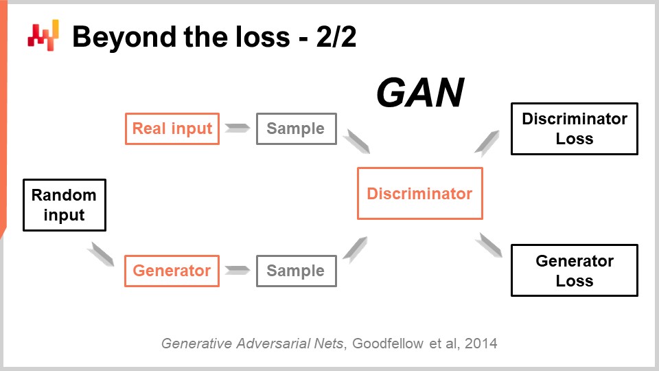
This very impressive achievement has been obtained with a beautifully simple technique called Generative Adversarial Networks (GANs). In the press, you may have heard of these techniques as deepfakes. Deepfakes are images that have been produced with this GAN technique. How does it work?
Well, the way it works is that you first start with a generator. The generator takes some noise as input, which are just random values, and it’s going to produce an image in the present case. If we are back to the supply chain case, it would produce trajectories for all the demand points observed for every single SKU for, let’s say, the next three months in this fashion store. This generator is itself a deep learning network.
Now, we are going to have a discriminator. A discriminator is also a deep learning network, and the goal of the discriminator is to learn whether to predict whether what has just been generated is real or synthetic. The discriminator is a binary classifier that just needs to say if it is real or not real. If the discriminator is able to correctly predict that a sample is fake, it’s synthetic, we are going to conduct the gradients back to the generator and let the generator learn from it.
What happens from this setup is that the generator starts learning how to generate samples that actually fool and confuse the discriminator. At the same time, the discriminator learns how to get better at discriminating between the real samples and the synthetic ones. If you take this process, it hopefully converges to a state where you end up with both a very high-quality generator that generates samples that are incredibly realistic, and a very good discriminator that can tell you whether it is real or not. This is exactly what is being done with GANs to generate those photorealistic pictures. If we go back to the supply chain, you will find experts in supply chain circles who say that for a particular situation, the best metric is MAPE, or weighted MAPE, or whatever. They will come up with recipes telling you that in certain situations, you need to use this metric or that one. The reality is that deep learning shows that a forecasting metric is an outdated concept. If you want to achieve high-dimensional accuracy, not just pointwise accuracy, you need to learn the metric. Although at the moment, I suspect there are next to zero supply chains that are leveraging these techniques, at some point in the future, they will be. It will become the norm to learn the forecasting metric using generative adversarial networks or the descendants of these techniques because it’s a way to capture the subtle, high-dimensional behavior that is truly of interest, instead of just having pointwise accuracy.
Now, so far, every single observation came with a label, and the label was the output we want to predict. However, there are situations that cannot be framed as input-output problems. Labels are simply not available. If we want to take a supply chain example, that would be an hypermarket. In hypermarkets, stock levels are not perfectly accurate. Goods can be damaged, stolen, or expired, and there are plenty of reasons why the electronic records in your system do not truly reflect what is available on the shelf as perceived by the customers. Inventorying is too expensive to be a real-time data source of accurate inventory. You can do inventorying, but you can’t run through the entire hypermarket every single day. What you end up with is a large amount of slightly inaccurate stock. You have tons of it, but you can’t really say which ones are accurate or not.
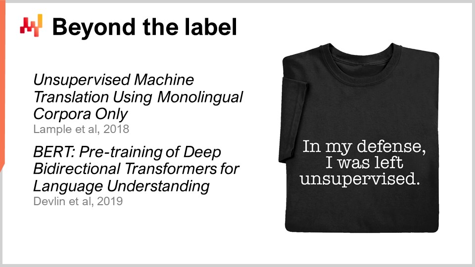
This is essentially the sort of situation where unsupervised learning really makes sense. We want to learn something; we have data, but we don’t have the right answers available. We don’t have those labels. What we have is just tons of data. Unsupervised learning has been considered for decades by the machine learning community as a holy grail. For a very long time, it was the future but a distant future. However, recently there have been some incredible breakthroughs in this area. One of the breakthroughs was, for example, accomplished by a Facebook team with a paper titled “Unsupervised Machine Translation Using Monolingual Corpora Only.”
What the Facebook team did in this paper was to build a translation system that only used a corpus of English text and a corpus of French text. These two corpora have nothing in common; it’s not even the same text. It’s just text in English and text in French. Then, without giving any actual translation to the system, they learned a system that translates from English to French. This is an absolutely stunning result. By the way, the way it’s accomplished is by using a technique that is incredibly reminiscent of the generative adversarial networks that I’ve just presented previously. Similarly, a team at Google published BERT (Bidirectional Encoder Representations from Transformers) two years ago. BERT is a model that is trained in a way that is largely unsupervised. We’re talking about text again. The way it’s done with BERT is by taking enormous databases of text and masking words randomly. Then, you train the model to predict those words and rinse and repeat for the entire corpus. Some people refer to this technique as self-supervised, but what is very interesting with BERT and where it becomes relevant for supply chain is that suddenly, the way you approach your data is to build a machine where you can hide parts of the data, and the machine is still able to re-complete the data.
The reason this is of prime relevance for supply chain is that fundamentally, what is being done with BERT in the context of natural language processing can be extended to many other domains. It’s the ultimate “what-if” answering machine. For example, what if I had one more store? This “what-if” can be answered because you can just modify your data, add the store, and query the machine learning model that you’ve just built. What if I had one extra product? What if I had one extra client? What if I had a different price point for this product? And so on. Unsupervised learning is of primary interest because you start treating your data as a whole, not just as a list of pairs. You end up with a mechanism that is completely general and can make predictions on any aspect that happens to be somewhat present in the data. This is very powerful.
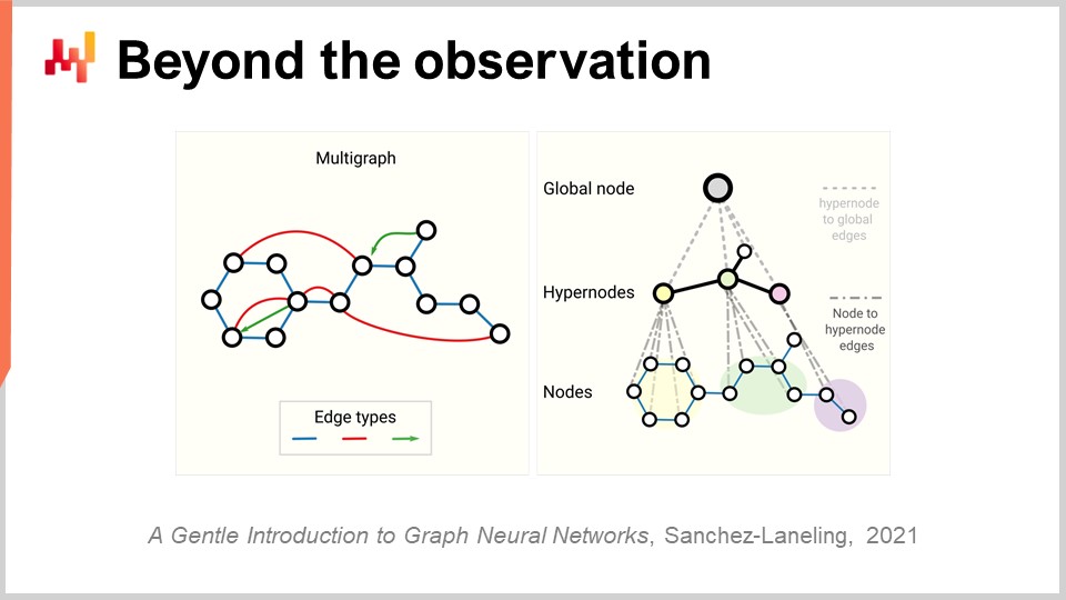
Now, finally, we have to revisit the whole concept of observation. Initially, we said that an observation was a pair of features plus a label. We have seen how we can remove the label, but what about the features themselves and the observation? The problem with supply chain is that we don’t really have observations. It’s not even clear that we can decompose a supply chain into a list of independent or homogeneous observations. As discussed in a previous lecture, what we have to observe a supply chain is not any direct scientific observation of the supply chain itself. What we have is a series of pieces of enterprise software, and the only way we can observe a supply chain is indirectly through the records collected into those pieces of enterprise software. That can be the ERP, the WMS, the point of sales, etc. But the bottom line is that all we have is essentially electronic records that are transactional in nature because all those systems are typically implemented on top of transactional databases. Thus, the observations are not independent. The records that we have are relational, quite literally, because they live in a relational database. When I say they have relations, I mean that if you look at a customer with a loyalty card, for example, they are connected to all the products they purchased. Every single product is connected to all the stores where the product is part of the assortment. Every single store is connected to all the warehouses that have the capacity to serve the store of interest. So, we don’t have independent observations; we have data with tons of relational structure overlaid on top of it, and none of those elements are truly independent from the others.
The relevant breakthrough in deep learning to tackle this sort of interconnected data is known as graph learning. Graph learning is exactly what you need to tackle behaviors like substitution and cannibalization in fashion. The best way to see cannibalization is to think that all the products are competing for the same clients, and by analyzing the data that connects clients and products, you can analyze cannibalization. Beware, graph learning has nothing to do with graph databases, which are something entirely different. Graph databases are essentially just databases used to query graphs, with no learning involved. Graph learning is about learning some extra properties about the graphs themselves. It’s about learning relationships that can or cannot be observed or that cannot be observed fully, or to decorate the sort of relationship that we have with an overlay of actionable knowledge.
My take is that due to the fact that by design, supply chain is a system where all the parts are interconnected – that’s the curse of supply chain, where you can’t just locally optimize anything without displacing problems – graph learning will become increasingly prevalent as an approach to tackle those problems in supply chain and machine learning. Essentially, graph neural networks are deep learning techniques designed to deal with graphs.
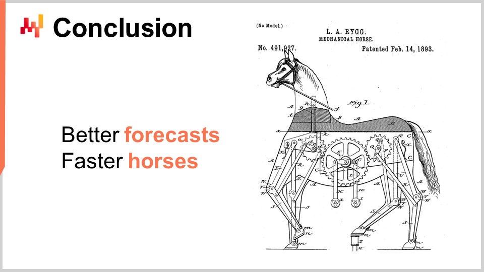
In conclusion, thinking that machine learning is about delivering more accurate forecasts is, to put it mildly, rather naive. It is like saying the main point of an automobile is to get access to a faster horse. Yes, it is true that most likely through machine learning, we can achieve more accurate forecasts. However, this is a small part of a very large picture, and a picture that keeps getting bigger as there are breakthroughs made in the machine learning community. We started with machine learning frameworks that included a series of concepts: feature, label, observation, model, and loss. This small, elementary framework was already vastly more general than the time series forecasting perspective. With the recent development of machine learning, we see that even those concepts are slowly and gradually fading into irrelevance due to the fact that we are discovering ways to transcend them. For supply chain, this paradigm shift is of critical importance because it means that we have to apply this same sort of paradigm shift when it comes to forecasting. Machine learning forces us to entirely rethink how to approach data and what we can do with data. Machine learning opens doors that were very firmly closed until very recently.
Now let’s have a look at some questions.
Question: Don’t random forests use bagging?
My point is that, yes, they are an extension of that, and there is more to them than just bagging. Bagging is an interesting technique, but whenever you see a machine learning technique, you have to ask yourself: is this technique going to make me progress toward my capacity to learn the really hard problems like cannibalization or substitution? And, is this sort of technique going to play well with the computing hardware that you have? This is one of the key takeaways you should take from this lecture.
Question: With the push for companies to have everything automated with robotics, what is the future of logistics warehouse workers? Will they be replaced by robots in the near future?
This question is not exactly related to machine learning, but it’s a very good question. Factories have undergone massive transformation toward extensive robotization, which may or may not use robots. Factories’ productivity has increased, and even now in China, factories are vastly automated for the most part. Warehouses were late to the party. However, what I see nowadays is the development of warehouses that are increasingly mechanical and automated. I would not say it’s necessarily robots; there are many competing technologies to build a warehouse that achieves a higher degree of automation. The bottom line is that the trend is clear. Warehouses and logistics centers, in general, are going to undergo the same sort of massive productivity improvement that we have already witnessed in production.
To answer your question, I’m not saying that people will be replaced by robots; they will be replaced by automation. Automation will sometimes take the form of something like a robot, but it can also take many other forms. Some of the forms are just clever setups that vastly improve productivity without involving the sort of technology that we intuitively associate with robots. However, I believe that the logistics part of supply chain overall is going to shrink. The only thing that keeps this rising right now is the fact that with the rise of e-commerce, we have to take care of the last mile. The last mile is increasingly occupying the bulk of the workforce that has to deal with logistics. Even the last mile is going to be automated in the not-so-distant future. Autonomous vehicles are just around the corner; they were promised for this decade, and although they might be arriving a bit late, they are coming.
Question: Do you think that machine learning is worth investing time to learn in order to work in supply chain?
Absolutely. In my opinion, machine learning is an auxiliary science of supply chain. Consider the relationship a physician has with chemistry. If you are a modern-day physician, nobody expects you to be a chemist. However, if you tell your patient that you know absolutely nothing about chemistry, people would think that you don’t have what it takes to be a modern physician. Machine learning should be approached in the same way people who study medicine approach chemistry. It’s not an end, but a means. If you want to do serious work in supply chain, you need to have solid foundations in machine learning.
Question: Could you give examples where you applied machine learning? Did the tool become operational?
Speaking for myself as Joannes Vermorel, the entrepreneur and CEO of Lokad, we have over 100 companies in production at the moment, all using machine learning for diverse tasks. These tasks include forecasting lead times, producing probabilistic forecasts of demand, predicting returns, predicting quality problems, revising estimates of mean time between unscheduled repairs, and detecting whether competitive prices are correct or not. There are many applications, such as reassessing compatibility matrices between cars and parts in the automotive aftermarket. With machine learning, you can fix a large portion of database errors automatically. At Lokad, not only do we have those 100 companies in production, but it has been the case for close to a decade now. The future is already here; it’s just not evenly distributed.
Question: What is the best way to learn machine learning on your own time? Would you recommend sites like Udemy, Coursera, or anything else?
My suggestion would be a combination of Wikipedia and reading papers. As you’ve seen in this lecture, it’s important to understand the fundamentals and stay up-to-date with the latest developments in the field. As you’ve seen in these lectures, I’m quoting actual research papers. Don’t trust second-hand information; go directly for what was published. All these things are directly available online. There are papers in machine learning that are poorly written and indecipherable, but there are also papers that are brilliantly written and provide crystal clear insights about what is going on. My suggestion is to go for Wikipedia for a high-level overview of a field, so that you can get the big picture, and then start reading papers. At first, it may seem opaque, but after a while, you’ll get used to it. You can go for Udemy or Coursera, but personally, I never did that. My goal when I do these lectures is to give you a few tidbits of intuition so that you get the big picture. If you want to go into the nitty-gritty detail, just jump into the actual paper that was published years or decades ago. Go for first-hand information, and trust your own intelligence.
Deep learning is a very empirical field of research. Most of the stuff being done isn’t extremely complex, mathematically speaking. It usually doesn’t go beyond what you learn at the end of high school, so it’s fairly accessible.
Question: With the rise of no-code tools like CodeX and Co-Pilot from OpenAI, do you see supply chain practitioners writing models in plain English at any point in time?
The short answer is: no, not at all. The idea that you could bypass coding has been around for a long time. For example, Microsoft’s Visual Basic was intended to be a visual tool so people wouldn’t have to program anymore; they could just visually compose stuff like Legos. But nowadays, this approach has proven to be ineffective, and the next trend is expressing things verbally.
However, the reason I use mathematical formulas in these lectures is that there are many situations where using a mathematical formula is the only way to convey clearly what you’re trying to say. The problem with the English language, or any natural language, is that it’s often imprecise and prone to misinterpretation. In contrast, mathematical formulas are precise and clear. The problem with plain language is that it’s incredibly fuzzy, and while it has its uses, the reason we employ formulas is to provide unambiguous meaning to what is being said. I try to make limited use of formulas, but when I include one, it’s because I feel it’s the only way to clearly convey the idea, with a level of clarity surpassing what I can say verbally.
Regarding low-code platforms, I’m very skeptical, as this approach has been attempted many times in the past without much success. My personal take is that we should make coding more appropriate for supply chain management by identifying why coding is hard and removing accidental complexity. What remains is coding done right for supply chain, which is what Lokad aims to do.
Question: Does machine learning make demand forecasting more accurate for seasonal or regular sales history data?
As I mentioned in this presentation, machine learning makes the concept of accuracy obsolete. If you look at the last large-scale time series forecasting competition, the M5 competition, the top 10 models were all machine learning models to some degree. So, does machine learning make forecasts more accurate? Factually, based on the forecasting competition, yes. But it’s only marginally more accurate compared to other techniques, and it’s not groundbreaking extra accuracy.
Moreover, you shouldn’t think of forecasting in a one-dimensional perspective. When you ask about accuracy for seasonality, you’re considering one product at a time, but that’s not the right approach. True accuracy is assessing how launching a new product affects all other products, as there will be some degree of cannibalization. The key is to evaluate whether the way you reflect this cannibalization in your model is accurate or not. Suddenly, this becomes a many-dimensional problem. As I presented in the lecture with generative networks, the metric of what accuracy actually means has to be learned; it cannot be given. Mathematical formulas, such as mean absolute error, mean absolute percentage error, and mean square error, are just mathematical criteria. They are not the sort of metrics we actually need; they are just very naive metrics.
Question: Will the mundane work of forecasters be replaced with forecasting in auto mode?
I would say the future is already here, but it’s not evenly distributed. At Lokad, we already forecast tens of millions of SKUs daily, and I don’t have anyone tuning any forecasts on the payroll. So yes, it is already being done, but this is just a small part of the picture. If you need to have people adjusting forecasts or tuning forecasting models, it indicates a dysfunctional approach. You should think of the need to tune forecasts as a bug and address it by automating that part of the process.
Again, from Lokad’s experience, these things will be entirely eliminated because we have already done it. We are not the only ones doing it this way, so for us, it is almost ancient history, being the case for almost a decade.
Question: How far is machine learning being actively used in making supply chain decisions?
It depends on the company. At Lokad, it’s used all over the place, and obviously, when I say “at Lokad,” I mean when in companies served by Lokad. However, the vast majority of the market is still essentially using Excel, with no machine learning whatsoever. Lokad is actively managing billions of euros or dollars worth of inventory, so that is already a reality and has been for quite a while. But Lokad is not even 0.1% of the market, so we are still an outlier. We are growing fast, as are quite a few competitors. My suspicion is that it’s still a fringe setup in the entire supply chain market, but it has double-digit growth. Never underestimate the power of exponential growth over a long period of time. Ultimately, it will get very big, hopefully with Lokad, but that is another story.
Question: With lots of unknowns in supply chain, what is a strategy that can make it assuming inputs for a model?
The idea is that, yes, there are tons of unknowns, but the inputs of your model are not really up for choice. It boils down to what you have in your enterprise systems, like what sort of data exists in your ERP. If your ERP has historical stock levels, then you can use them as part of your machine learning model. If your ERP only keeps current stock levels, then this data is not available. You can start to snapshot your stock levels if you want to use that as extra inputs, but the core message is that there is very little choice involved in what you can use as inputs; it’s literally what exists in your systems.
My typical approach is that if you have to create new data sources, it’s going to be sluggish and painful, and that’s probably not going to be your starting point for using machine learning in supply chains. Larger companies have been digitalized for decades, so what you have in your transactional systems, like your ERP and WMS, is already an excellent starting point. If down the road, you realize that you want to have more, such as competitive intelligence, authorized stock levels, or ETAs given by your suppliers, those will be worthy additions to use as inputs for your models. Usually, what you use as inputs is something that you have a good intuition correlates with whatever you’re trying to predict in the first place, and high-level intuition is usually enough. Common sense, which is hard to define, is vastly sufficient. This is not the bottleneck in terms of engineering.
Question: What is the impact of pricing decisions on the estimation of future demand, even in a probabilistic perspective, and how to deal with it from a machine learning perspective?
This is a very good question. There was an episode on LokadTV that addressed this very problem. The idea is that what you learn becomes what is typically known as a policy, an object that controls the way you react to various events. The way you forecast is to produce a sort of landscape, Monte Carlo style. You’re going to produce a trajectory, but your forecast will not be static data points. It’s going to be a much more generative process, where at every stage of the forecasting process, you’ll have to generate the sort of demand that you can observe, generate the decisions that you take, and regenerate the sort of market response to what you just did.
It becomes very complicated to assess the accuracy of your demand response generating process, and that’s why you need to actually learn your forecasting metrics. That is very tricky, but that’s why you can’t just think of your forecasting metrics, your accuracy metrics, as a one-dimensional problem. To summarize, demand forecasting becomes a generator, so it’s fundamentally dynamic, not static. It’s something that is generative. This generator reacts to an agent, an agent that is going to be implemented as a policy. Both the generator and the policy-making system have to be learned. You also have to learn the loss function. There’s a lot to learn, but fortunately, deep learning is a very modular and programmatic approach that lends itself well to the composition of all these techniques.
Question: Is it difficult to collect data, especially from SMEs?
Yes, it is very difficult. The reason is that, if you’re dealing with a company that has less than 10 million in turnover, there is no such thing as an IT department. There might be a small ERP in place, but even if the tools are good, decent, and modern, you don’t have an IT team in place. When you ask for the data, there is nobody in the client company that has the competency to run a SQL query to extract the data.
I’m not sure if I understand your question correctly, but the problem is not exactly collecting the data. Collecting the data is done naturally through the accounting software or the ERP that is in place, and nowadays, you have ERPs accessible even to fairly small companies. The problem is the extraction of data from those pieces of enterprise software. If you’re with a company that has less than 20 million dollars in turnover and they are not an e-commerce company, chances are the IT department is nonexistent. Even when there is a tiny IT department, it’s usually just one person responsible for setting up machines and Windows desktops for everybody. It’s not someone who is familiar with databases and more advanced administrative tasks in terms of IT setups.
Okay, I guess this is it. The next session will be a couple of weeks from now. It will be on Wednesday, the 13th of October. See you next time!
References
- A theory of the learnable, L. G. Valiant, November 1984
- Support-vector networks, Corinna Cortes, Vladimir Vapnik, September 1995
- Random Forests, Leo Breiman, October 2001
- LightGBM: A Highly Efficient Gradient Boosting Decision Tree, Guolin Ke, Qi Meng, Thomas Finley, Taifeng Wang, Wei Chen, Weidong Ma, Qiwei Ye, Tie-Yan Liu, 2017
- Attention Is All You Need, Ashish Vaswani, Noam Shazeer, Niki Parmar, Jakob Uszkoreit, Llion Jones, Aidan N. Gomez, Lukasz Kaiser, Illia Polosukhin, last revised December 2017
- Deep Double Descent: Where Bigger Models and More Data Hurt, Preetum Nakkiran, Gal Kaplun, Yamini Bansal, Tristan Yang, Boaz Barak, Ilya Sutskever, December 2019
- Analyzing and Improving the Image Quality of StyleGAN, Tero Karras, Samuli Laine, Miika Aittala, Janne Hellsten, Jaakko Lehtinen, Timo Aila, last revised March 2020
- Generative Adversarial Networks, Ian J. Goodfellow, Jean Pouget-Abadie, Mehdi Mirza, Bing Xu, David Warde-Farley, Sherjil Ozair, Aaron Courville, Yoshua Bengio, June 2014
- Unsupervised Machine Translation Using Monolingual Corpora Only, Guillaume Lample, Alexis Conneau, Ludovic Denoyer, Marc’Aurelio Ranzato, last revised April 2018
- BERT: Pre-training of Deep Bidirectional Transformers for Language Understanding, Jacob Devlin, Ming-Wei Chang, Kenton Lee, Kristina Toutanova, last revised May 2019
- A Gentle Introduction to Graph Neural Networks, Benjamin Sanchez-Lengeling, Emily Reif, Adam Pearce, Alexander B. Wiltschko, September 2021
