00:01 Introduction
01:56 The M5 uncertainty challenge - Data (1/3)
04:52 The M5 uncertainty challenge - Rules (2/3)
08:30 The M5 uncertainty challenge - Results (3/3)
11:59 The story so far
14:56 What is (probably) about to happen
15:43 Pinball loss - Foundation 1/3
20:45 Negative binomial - Foundation 2/3
24:04 Innovation Space State Model (ISSM) - Foundation 3/3
31:36 Sales structure - The REMT model 1/3
37:02 Putting it together - The REMT model 2/3
39:10 Aggregated levels - The REMT model 3/3
43:11 Single stage learning - Discussion 1/4
45:37 Pattern complete - Discussion 2/4
49:05 Missing patterns - Discussion 3/4
53:20 Limits of the M5 - Discussion 4/4
56:46 Conclusion
59:27 Upcoming lecture and audience questions
Description
In 2020, a team at Lokad achieved No5 over 909 competing teams at the M5, a worldwide forecasting competition. However, at the SKU aggregation level, those forecasts landed No1. Demand forecasting is of primary importance for supply chain. The approach adopted in this competition proved to be atypical, and unlike the other methods adopted by the other top 50 contenders. There are multiple lessons to be learned from this achievement as a prelude to tackle further predictive challenges for supply chain.
Full transcript
Welcome to this series of supply chain lectures. I’m Joannes Vermorel, and today I will be presenting “Number One at the SKU Level in the M5 Forecasting Competition.” An accurate demand forecast is considered as one of the pillars of supply chain optimization. Indeed, every single supply chain decision reflects a certain anticipation of the future. If we can gather superior insights about the future, then we can derive decisions that are quantitatively superior for our supply chain purposes. Thus, identifying models that deliver state-of-the-art predictive accuracy is of primary importance and interest for supply chain optimization purposes.
Today, I will be presenting a simple sales forecasting model that, despite its simplicity, ranked number one at the SKU level in a worldwide forecasting competition known as the M5, based on a dataset provided by Walmart. There will be two goals for this lecture. The first goal will be to understand what it takes to achieve state-of-the-art forecasting sales accuracy. This understanding will be of foundational interest for later efforts at predictive modeling. The second goal will be to set the right perspective when it comes to predictive modeling for supply chain purposes. This perspective will also be used to guide our later progression in this area of predictive modeling for supply chain.
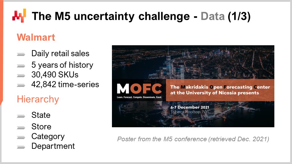
The M5 was a forecasting competition that took place in 2020. This competition is named after Spyros Makridakis, a notable researcher in the field of forecasting. This was the fifth edition of this competition. These competitions happen every couple of years and tend to vary in terms of focus depending on the type of dataset that is used. The M5 was a supply chain-related challenge, as the dataset used was retail store data provided by Walmart. The M6 challenge, which is yet to happen, will be focusing on financial forecasting.
The dataset used for the M5 was and remains a public dataset. It was Walmart retail store data aggregated at the daily level. This dataset included about 30,000 SKUs, which, retail-wise, is a fairly small dataset. Indeed, as a rule of thumb, a single supermarket typically holds about 20,000 SKUs, and Walmart operates over 10,000 stores. Thus, overall, this dataset – the M5 dataset – was about less than 0.1% of the worldwide Walmart-scale dataset that would be relevant from a supply chain perspective.
Moreover, as we will see in the following, there were entire classes of data that were missing from the M5 dataset. As a result, my approximate estimation is that this dataset is actually closer to 0.01% of the scale of what it would take at the scale of Walmart. Nevertheless, this dataset is plenty enough to do a very solid benchmark of forecasting models in a real-world setup. In a real-world setup, we would have to pay close attention to scalability concerns. However, from the perspective of a forecasting competition, it is fair to make the dataset small enough so that most methods, even the widely inefficient methods, can be used in the forecasting competition. Also, it ensures that contenders are not limited by the amount of computing resources that they can actually throw at this forecasting competition.

The M5 competition included two distinct challenges known as Accuracy and Uncertainty. The rules were simple: there was a public dataset that every participant could access, and in order to participate in one or both of these challenges, each participant had to produce a dataset of its own, which was its forecast dataset, and submit that to the Kaggle platform. The Accuracy challenge was about delivering an average time series forecast, which is the most classic sort of formal forecast. In this specific situation, it was about delivering a daily average forecast for about 40,000-time series. The Uncertainty challenge was about delivering quantile forecasts. Quantiles are forecasts with a bias; however, the bias is intentional. This is the whole point of having quantiles. This lecture focuses exclusively on the Uncertainty challenge, and the reason is that in supply chain, it’s the unexpectedly high demand that creates stockouts, and it’s the unexpectedly low demand that creates inventory write-offs. Costs in supply chains are concentrated at the extremes. This is not the average that interests us.
Indeed, if we look at what the average even means in the situation of Walmart, it turns out that for most products, in most stores, for most days, the average sales that are going to be observed is zero. Thus, most products have a fractional average forecast. Such average forecasts are very underwhelming as far as supply chain is concerned. If your options are either to store zero or replenish one unit, average forecasts are quite of little relevance. Retail is not in a unique position here; it is pretty much the same sort of situation whether we are discussing FMCG, aviation, manufacturing, or luxury – practically every single other vertical.
Back to the M5 Uncertainty challenge, there were four quantiles to be produced, respectively at 50%, 67%, 95%, and 99%. You can think of those quantile targets as service-level targets. The accuracy of those quantile forecasts was scored against a metric known as a pinball loss function. I will be getting back to this error metric later on in this lecture.
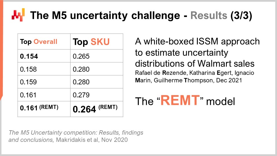
There were 909 teams competing worldwide in this Uncertainty challenge. A team from Lokad did rank number five overall, but number one at the SKU level. Indeed, while SKUs represented about three-quarters of the time series in this challenge, there were various aggregation levels ranging from the state (as in the United States – Texas, California, etc.) to the SKU, and all the aggregation levels were equi-weighted in the final score of this competition. Thus, even if SKUs were about three-quarters of the time series, they were only about 8% of the total weight in the final score of the competition.
The method used by this team from Lokad was published in a paper titled “A White Box ISSM Approach to Estimate Uncertainty Distribution of Walmart’s Sales.” I will be putting a link to this paper in the description of this video after this lecture is complete. You will find all the elements in greater detail. For the sake of clarity and concision, I will be referring to the model presented in this paper as the BRAMPT model, simply named after the initials of the four co-authors.
On the screen, I’ve listed the top five results for the M5, obtained from a paper that provides general insights on the outcome of this forecasting competition. The fine print of the rank is quite dependent on the chosen metric. This is not overly surprising. The Uncertainty challenge used a scaled flavor of the pinball loss function. We’ll be getting back to this error metric in a minute. Although the M5 Uncertainty challenge demonstrated that we don’t have the means to eliminate uncertainty with the forecasting methods we have, not even close, it is not at all a surprising result. Considering that retail store sales tend to be erratic and intermittent, it emphasizes the importance of embracing uncertainty instead of just dismissing it entirely. However, it is remarkable to note that supply chain software vendors were all absent from the top 50 ranks of this forecasting competition, which is all the more intriguing considering that those vendors boast supposedly superior state-of-the-art forecasting technology of their own.

Now, this lecture is a part of a series of supply chain lectures. This present lecture is the first of what will be my fifth chapter in this series. This fifth chapter will be dedicated to predictive modeling. Indeed, gathering quantitative insights is necessary to optimize a supply chain. Whenever a supply chain decision is made – whether it’s deciding to buy materials, produce a certain product, move stock from one place to another, or increase or decrease the price of something you sell – this decision comes with a certain anticipation of future demand. Marginally, every single supply chain decision comes with a built-in expectation about the future. This expectation can be implicit and hidden. However, if we want to improve the quality of our expectation about the future, we need to reify this expectation, which is typically done through a forecast, although it doesn’t necessarily have to be a time series forecast.
The fifth and present chapter is named “Predictive Modeling” rather than “Forecasting” for two reasons. First, forecasting is almost invariably associated with time series forecasting. However, as we will see in this chapter, there are many supply chain situations that don’t really lend themselves to the time series forecasting perspective. Thus, in this regard, predictive modeling is a more neutral term. Second, it’s modeling that holds the true insight, not the models. We are looking for modeling techniques, and it’s through these techniques that we can expect to be able to cope with the sheer diversity of situations encountered in real-world supply chains.
The present lecture serves as a prologue for our predictive modeling chapter to establish that predictive modeling isn’t some kind of wishful thinking about forecasting, but that it qualifies as a state-of-the-art forecasting technique. This comes on top of all the other benefits that will gradually become clear as I progress through this chapter.
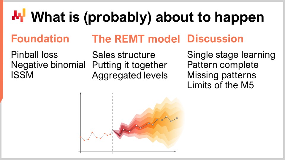
The rest of this lecture will be organized in three parts. First, we will review a series of mathematical ingredients, which are essentially the building blocks of the BRAMPT model. Second, we will assemble those ingredients in order to construct the BRAMPT model, just as it was during the M5 competition. Third, we will discuss what can be done to improve upon the BRAMPT model and also to see what could be done to improve upon the forecasting challenge itself, as it was presented in the M5 competition.
The Uncertainty challenge of the M5 seeks to compute quantile estimates of future sales. A quantile is a point in a one-dimensional distribution, and by definition, a 90 percent quantile is the point where there is a 90 percent chance to be below this quantity value and a 10 percent chance to be above it. The median is, by definition, the 50 percent quantile.
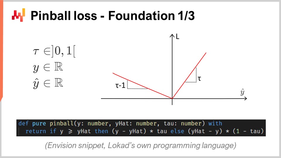
The pinball loss function is a function with a deep affinity for quantiles. Essentially, for any given tau value between zero and one, tau can be interpreted, from a supply chain perspective, as a service level target. For any tau value, the quantile associated with tau happens to be the value within the probability distribution that minimizes the pinball loss function. On the screen, we see a straightforward implementation of the pinball loss function, written in Envision, the domain-specific programming language of Lokad dedicated to supply chain optimization purposes. The syntax is fairly Python-like and should be relatively transparent to the audience.
If we try to unpack this code, we have y, which is the real value, y-hat, which is our estimate, and tau, which is our quantile target. Again, the quantile target is fundamentally the service level target in supply chain terms. We see that the under forecast comes with a weight equal to tau, while the over forecast comes with a weight equal to one minus tau. The pinball loss function is a generalization of the absolute error. If we go back to tau equals 0.5, we can see that the pinball loss function is just the absolute error. If we have an estimate that minimizes the absolute error, what we get is an estimation of the median.
On the screen, you can see a plot of the pinball loss function. This loss function is asymmetric, and through an asymmetric loss function, we can get not the average or median forecast, but a forecast with a controlled bias, which is exactly what we want to have for a quantile estimate. The beauty of the pinball loss function is its simplicity. If you have an estimate that minimizes the pinball loss function, then you have a quantile forecast by construction. Thus, if you have a model that has parameters and you steer the optimization of the parameters through the lenses of the pinball loss function, what you will get out of your model is essentially a quantile forecasting model.
The M5 Uncertainty challenge presented a series of four quantile targets at 50, 67, 95, and 99. I typically refer to such a series of quantile targets as a quantile grid. A quantile grid, or quantized grid forecasts, are not quite probabilistic forecasts; it’s close, but not there yet. With a quantile grid, we are still cherry-picking our targets. For example, if we said that we want to produce a quantile forecast for the 95 percent, the question becomes, why 95, why not 94 or 96? This question is left unanswered. We will have a closer look at that later on in this chapter, but not in this lecture. Let’s suffice to say that the main gain we have with probabilistic forecasts is to eliminate entirely this cherry-picking aspect of the quantile grids.
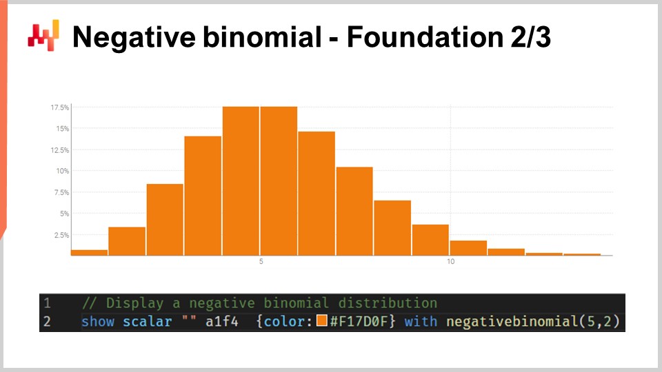
Most of the audience is probably familiar with the normal distribution, the Gaussian bell-shaped curve that occurs very frequently in natural phenomena. A count distribution is a distribution of probabilities over every integer. Unlike continuous real distributions like the normal distribution that gives you a probability for every single real integer, count distributions only care about non-negative integers. There are many classes of count distributions; however, today our interest lies in the negative binomial distribution, which is used by the REM model.
The negative binomial distribution comes with two parameters, just like the normal distribution, which also effectively control the mean and the variance of the distribution. If we choose the mean and the variance for a negative binomial distribution so that the bulk of the mass of the probability distribution is far from zero, we have a behavior for the negative binomial distribution that asymptotically converges to a normal distribution behavior if we were to collapse all the probability values toward the nearest integers. However, if we look at distributions where the mean is small, especially compared to the variance, we will see that the negative binomial distribution starts to significantly diverge in terms of behavior compared to a normal distribution. In particular, if we look at small mean negative binomial distributions, we will see that these distributions become highly asymmetric, unlike the normal distribution, which remains completely symmetric no matter which mean and variance you pick.
On the screen, a negative binomial distribution is plotted through Envision. The line of code that was used to produce this plot is on display below. The function takes two arguments, which is expected as this distribution has two parameters, and the result is just a random variable that gets displayed as a histogram. I am not going to delve into the fine print of the negative binomial distribution here in this lecture. This is straightforward probability theory. We have explicit closed-form analytical formulas for the mode, the median, the cumulative distribution function, skewness, kurtosis, etc. The Wikipedia page gives you a pretty decent summary of all those formulas, so I invite the audience to have a look if they want to know more about this specific kind of count distribution.
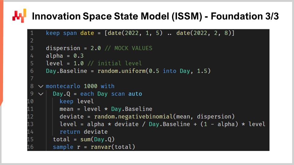
Let’s move to the Innovation Space State Model, or ISSM. The innovation space state model is a long and impressive-sounding name to do something that is quite simple. In fact, the ISSM is a model that transforms a time series into a random walk. With ISSM, you can turn just a plain vanilla time series forecast, and when I say average, I mean a forecast where for each period you will have one value set at the average, into a probabilistic forecast, and not just a quantile forecast but directly a probabilistic forecast. On the screen, you can see a complete ISSM implementation written once again in Envision. We can see that it’s only a dozen or so lines of code, and actually, most of those lines of code are not even doing much. ISSM is literally very straightforward, and it would be very straightforward to re-implement this piece of code into any other language, such as Python.
Let’s have a closer look at the fine print of those lines of code. In line one, I am specifying the range of the periods where the random walk will happen. From the perspective of the M5, we want a random walk for a period of 28 days, so we have 28 points, one point per day. At lines three, four, and five, we introduce a series of parameters that will control the random walk itself. The first parameter is the dispersion, which will be used as an argument to control the shape of the negative binomials that occur inside the ISSM process. Then we have alpha, which is essentially the factor that controls the exponential smoothing process that also happens inside the ISSM. At line five, we have the level, which is just the initial state of the random walk. Finally, at line six, we have a series of factors which are typically intended to capture all the calendar patterns that we want to embed in our forecasting model.
Now, the values from lines three to six just come with mock initialization. For the sake of concision, I will get to how those values are actually optimized in a minute, but here all the initialization that you see are just mock values. I’m just even drawing random values for the baseline. We will get to how, in reality, if you want to use this model, you will need to properly initialize those values, which we will do later in this lecture.
Now let’s have a look at the core of the ISSM process. The core starts at line eight and it starts with a loop of 1000 iterations. I just said that the ISSM process is a process to generate random walks, so here we are doing 1000 iterations, or we are going to do 1000 random walks. We could have more, we could have less; it is a straightforward Monte Carlo process. Then at line nine, we are doing a second loop. This is the loop that iterates one day at a time for the period of interest. So we have the outer loop, which is essentially one iteration per random walk, and then we have the inner loop, which is one iteration, just moving from one day to the next within the random walk itself.
At line 10, we have a keep level. To keep the level, just say that this parameter is going to be mutated within the inner loop, not within the outer loop. So that means that the level is something that varies when we go from one day to the next, but when we go from one random walk to the next through the Monte Carlo loop, this level is going to be reset to its initial value that is declared above. At line 11, we compute the mean. The mean is the second parameter that we use to control the negative binomial distribution. So we have the mean, we have the dispersion, and we have a negative binomial distribution. At line 12, we draw a deviate according to the normal binomial distribution. Drawing a deviate just means we take a random sample extracted from this count distribution. Then at line 13, we update this level based on the deviate that we have seen, and the update process is just a very simple exponential smoothing process, guided by the alpha parameter. If we take alpha very large, equal to one, that means we put all the weight on the last observation. On the contrary, if we were to put alpha equal to zero, it would mean that we would have zero drift; we would stay true to the original time series as defined in the baseline.
By the way, in Envision, when it’s written “.baseline,” what we see here is that there is a table, so it’s a table that has, let’s say, NDM5; that would have 28 values, and baseline is just a vector that belongs to this table. At line 15, we collect all the deviates and sum them through “someday.q.” We send them into a variable named “total,” so within one random walk, we have the total of the deviates that were collected for every single day. Thus, we have the total of the sales for 28 days. Finally, at line 16, we are essentially gathering and collecting those samples into a “render.” A render is a specific object in Envision, which is essentially a probability distribution of relative integers, positive and negative.
In summary, what we have is the ISSM as a random generator of one-dimensional random walks. In the context of sales forecasting, you can think of those random walks as possible future observations for the sales themselves. It’s interesting because we don’t think of the forecast as the average or the median; we literally think of our forecast as one possible instance of one future.
At this point, we have gathered everything that we need to start assembling the REMT model, which we are going to do now.
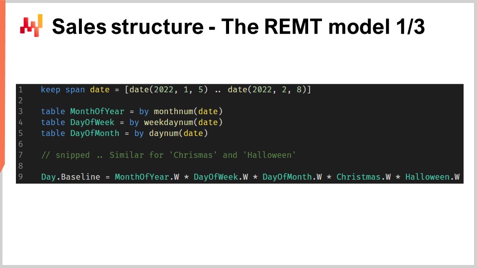
The REMT model adopts a multiplicative structure, which is reminiscent of the Holt-Winters forecasting model. Every day gets a baseline, which is a single value that happens to be the product of five calendar effects. We have, namely, the month of the year, the day of the week, the day of the month, Christmas, and Halloween effects. This logic is implemented as a concise Envision script.
Envision has a relational algebra that offers broadcast relationships between tables, which are very practical for this situation. The five tables that we have constructed, one table per calendar pattern, are constructed as grouping tables. So, we have the date table, and the date table has a primary key called “date.” When we write that we declare a new table with a “by” aggregation and then we have the date, what we are building is a table that has a direct broadcast relationship with the date table.
If we look specifically at the day of week table at line four, what we are building is a table that will have exactly seven lines. Each line of the table will be associated with one and only one line of the day of week. Thus, if we put values in this day of week table, we can broadcast those values quite naturally because every line on the recipient side, on the date side, will have one line to match in this day of week table.
At line nine, with vector “de.dot.baseline,” it is computed as the plain multiplication of the five factors on the right side of the assignment. All those factors are first broadcast to the date table, and then we proceed with a simple line-wise multiplication for every single line in the date table.
Now, we have a model that has a few dozen parameters. We can count those parameters: we have 12 parameters for the month of the year, from 1 to 12; we have seven parameters for the day of the week; and we have 31 parameters for the day of the month. However, in the case of NDM5, we are not going to learn one parameter value for all those values for every single SKU, as we would end up with a massively large number of parameters that would most likely vastly overfit the Walmart dataset. Instead, at NDM5, what was done was to leverage a trick known as parameter sharing.
Parameter sharing means that instead of learning distinct parameters for every single SKU, we are going to establish subgroups and then learn those parameters at the subgroup level. Then, we use the same values within those groups for those parameters. Parameter sharing is a very classic technique that is extensively used in deep learning, although it predates deep learning itself. During the M5, the month of year and day of week were learned at the store department aggregation level. I will get back to the various aggregation levels of the M5 in a second. The day-of-month value was actually hardcoded factors that were set at the state level, and when I say the state, I’m referring to the United States, such as California, Texas, etc. During the M5, all those calendar parameters were simply learned as direct averages over their related scopes. It’s a very direct way to set those parameters: you just take all the SKUs that belong to the same scope, average everything, normalize, and there you have your parameter.
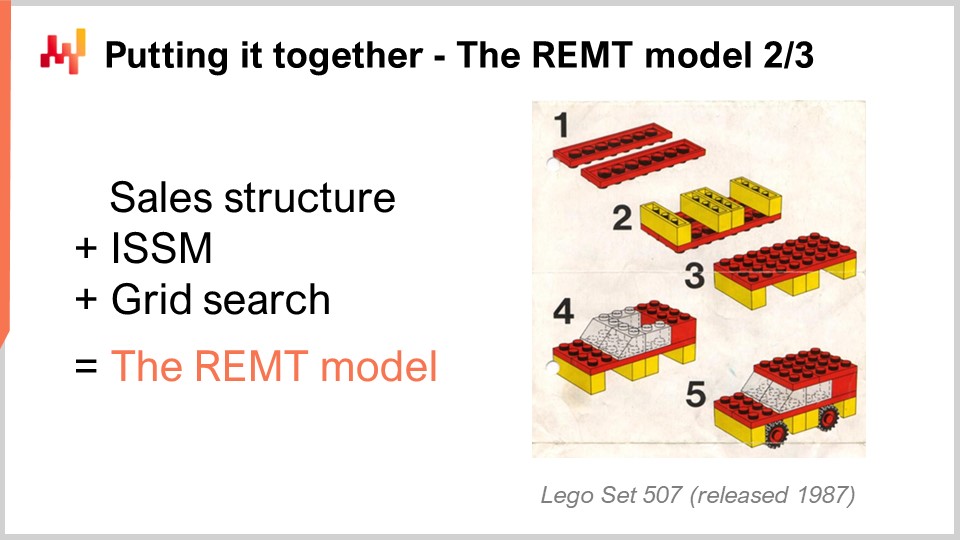
Now, at this point, we have gathered everything to assemble the REMT model. We have seen how to build the daily baseline, which embeds all the calendar patterns. The calendar patterns have been learned through direct averages of a certain scope, which is a crude but effective learning mechanism. We have also seen that the ISSM transforms a time series into a random walk. We are only left with establishing the proper values for the ISSM parameters, namely alpha, the parameter used for the exponential smoothing process that happened inside the SSM; the dispersion, which is a parameter used to control the negative binomial distribution; and the initial value for the level, which is used to initialize our random walk.
During the M5 competition, the team from Lokad leveraged a simple grid search optimization to learn those remaining three parameters. Grid search essentially means that you iterate over all the possible combinations of those values, going through small increments at a time. Grid search was directed using the pinball loss function, which I’ve previously described, to steer the optimization of those three parameters. For each SKU, grid search is probably one of the most inefficient forms of mathematical optimization. However, considering that we have only three parameters and that we only need to perform one optimization per time series, and that the M5 dataset itself is fairly small, it was suitable for the M5 competition.
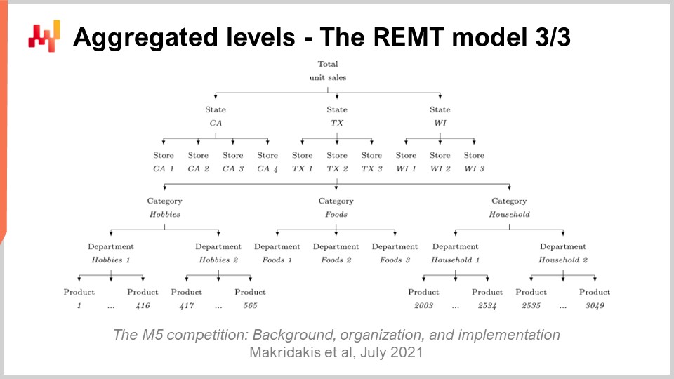
So far, we have presented how the REMT model operates at the SKU level. However, in the M5, there were 12 distinct aggregation levels. The SKU level, being the most disaggregated level, was the most important. A SKU, or stock-keeping unit, is literally one product in one location. If you have the same product in 10 locations, then you have 10 SKUs. Although the SKU is arguably the most relevant aggregation level for a supply chain, nearly all inventory-related decisions, such as replenishment and assortment, happen at the SKU level. The M5 was primarily a forecasting competition, and thus there was a lot of emphasis on the other aggregation levels.
On the screen, these levels summarize the aggregation levels that were present in the M5 dataset. You can see that we have the states, such as California and Texas. In order to deal with the higher aggregation levels, two techniques were used by the team from Lokad: either summing the random walks, meaning you perform the random walks at a lower aggregation level, sum them, and then achieve random walks at a higher aggregation level; or restarting the learning process entirely, directly jumping to the higher aggregation level. In the M5 uncertainty challenge, the REMT model was the best at the SKU level, but it wasn’t the best at the other aggregation levels, although it performed well overall across the board.
My own working hypothesis on why the REMT model was not the best at all levels is as follows (please note that this is a hypothesis and we didn’t actually test it): The negative binomial distribution offers two degrees of freedom through its two parameters. When looking at fairly sparse data, as found at the SKU level, two degrees of freedom strike the right balance between underfitting and overfitting. However, as we move toward higher aggregation levels, the data becomes denser and richer, so the trade-off probably shifts toward something better suited to capture more precisely the shape of the distribution. We would need a few extra degrees of freedom – likely just one or two extra parameters – to achieve this.
I suspect that increasing the degree of parametrization of the count distribution used at the core of the REMT model would have gone a long way to achieve something very close, if not directly state-of-the-art, for the higher aggregation levels. Nevertheless, we didn’t have time to do that, and we may revisit the case at some point in the future. This concludes what was done by the team at Lokad during the M5 competition.

Let’s discuss what could have been done differently or better. Even though the REMT model is a low-dimensional parametric model with a simple multiplicative structure, the process used to obtain the values of the parameters during the M5 was somewhat accidentally complicated. It was a many-stage process, with each calendar pattern having its own ad hoc special treatment, ending with a bespoke grid search to complete the REMT model. The whole process was quite time-consuming for data scientists, and I suspect it would be quite unreliable in production settings due to the sheer amount of ad hoc code involved.
In particular, my take is that we can and should unify the learning process of all the parameters as a single-stage process or, at the very least, unify the learning process so that the same method is used repeatedly. Nowadays, Lokad is using differentiable programming to do exactly that. Differentiable programming removes the need for ad hoc aggregations as far as the calendar patterns are concerned. It also removes the problem of precisely ordering the extraction of the calendar patterns by extracting all the patterns in one go. Finally, as differentiable programming is an optimization process of its own, it replaces the grid search with a much more efficient optimization logic. We will be reviewing how differentiable programming can be used for predictive modeling in the context of supply chain purposes in greater detail in later lectures in this chapter.
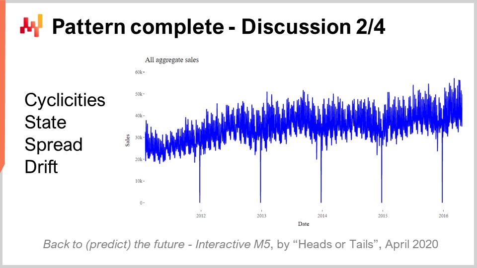
Now, one of the most surprising results of the M5 competition was that no statistical pattern remained unnamed. We had literally four patterns: simplicities, state, spread, and drift, which were all it took to achieve state-of-the-art forecasting accuracy in the M5 competition.
Simplicities are all calendar-based and none of them is even remotely surprising. The state can be represented as a single number that represents the level achieved by the SKU at a specific point in time. The spread can be represented with a single number that is the dispersion used to parameterize the negative binomial, and the drift can be represented with a single number associated with the exponential smoothing process that occurred within the SSM. We didn’t even have to include the trend, which was too weak for a 28-day horizon.
While we look at the total five years of aggregate sales for the M5 as displayed on the screen, the aggregation clearly shows a modest upward trend. Nevertheless, the REMT model operates without it and had zero consequences in terms of accuracy. The performance of the REMT model begs the question: is there any other pattern to capture, and have we missed any patterns?
At the very least, the performance of the REMT model shows that none of the more sophisticated models involved in this competition, such as gradient boosting trees or deep learning methods, captured anything beyond those four patterns. Indeed, if any of those models had managed to substantially capture anything, they would have vastly outperformed the REMT model at the SKU level, which they did not. The same can be said about all the more sophisticated statistical methods like ARIMA. Those models also failed to capture anything beyond what this very simple multiplicative parametric model has captured.
The Occam’s razor principle tells us that, unless we can find a very good reason to think that a pattern eludes us or a very good reason for some very interesting property that trumps the simplicity of this model, we don’t have any reason to use anything but a model that is at least as simple as the REMT model.
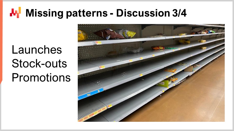
However, a series of patterns were absent from the M5 competition due to the very design of the M5 dataset. Those patterns are important, and in practice, any model that ignores them is going to work badly in a real retail environment. I’m basing this statement on my own experience.
First, we have the product launches. The M5 competition only included products that had at least five years’ worth of sales history. This is an unreasonable assumption as far as supply chain is concerned. Indeed, FMCG products typically have a lifespan of only a couple of years, and thus in an actual store, there is always a significant portion of the assortment that has less than one year’s worth of sales history. Furthermore, when looking at products with long lead times, numerous supply chain decisions have to be taken even before the product has a chance to be sold even once in any store. Thus, we need forecasting models that can even operate with zero sales history for a given product.
The second pattern of critical importance is stockouts. Stockouts occur in retail, and the M5 competition dataset ignored them entirely. However, stockouts cap sales. If a product is out of stock in the store, it will not be sold that day, and thus stockouts introduce a significant bias in the sales that we observe. The problem in the case of Walmart and general merchandise stores is even more complicated because the electronic records that capture the stock-on-hand values cannot be fully trusted. There are numerous inventory inaccuracies, and this needs to be taken into account as well.
Third, we have promotions. The M5 competition did include historical pricing; however, the price data was not provided for the period to be forecast. As a result, it appears that no contender in this competition managed to leverage the price information to improve forecasting accuracy. The REMT model does not use pricing information at all. Beyond the fact that we were missing the price information for the period of the forecast, promotions are not just about pricing. A product can be promoted by being prominently displayed in a store, which can significantly boost demand, regardless of whether the price has been lowered. Additionally, with promotions, we need to consider cannibalization and substitution effects.
Overall, the M5 dataset, from a supply chain perspective, can be seen as a toy dataset. While it remains probably the best public dataset in existence for carrying out supply chain benchmarks, it is still nowhere near something that would be truly equivalent to an actual production setup in even a modestly-sized retail chain.

However, the limitations of the M5 competition are not just due to the dataset. From a supply chain perspective, there are fundamental problems with the rules used to conduct the M5 competition.
The first fundamental problem is not to confuse sales with demand. We have already touched on this issue with stockouts. From a supply chain perspective, the true interest lies in anticipating demand, not sales. However, the problem goes deeper. The proper estimation of demand is fundamentally an unsupervised learning problem. It is not because arbitrary choices have been made about the applicable assortment in a store that the demand for a product should not be estimated. We must estimate the demand for products, irrespective of whether they are part of the assortment in any given store.
The second aspect is that quantile forecasts are less useful than probabilistic forecasts. Cherry-picking service levels leaves gaps in the picture, and quantile forecasts are relatively weak in terms of supply chain usage. A probabilistic forecast delivers a much more complete vision because it provides the complete probability distribution, eliminating this class of problems. The only key downside of probabilistic forecasts is that they require more tooling, especially when it comes to actually doing anything with the forecast downstream after the forecast has been produced. By the way, the REMT model actually delivers something that qualifies as a probabilistic forecast because, through the Monte Carlo process, you can generate an entire probability distribution. You just have to tune the number of Monte Carlo iterations.
In retail, customers don’t really care about the SKU perspective or the service level that can be achieved on any given SKU. The perception of customers in a general merchandise store like Walmart is driven by the basket. Typically, customers walk into a Walmart store with an entire shopping list in mind, not just one product. Additionally, there are tons of substitutes available in the store. The problem of using a single SKU metric to assess the quality of service is that it completely misses what customers perceive as quality of service in the store.
In conclusion, as a time series forecasting benchmark, the M5 competition is solid in terms of datasets and methodology. However, the time series perspective itself is lacking as far as supply chain is concerned. Time series do not reflect data as they are found in supply chains, nor do they reflect problems as they present themselves in supply chains. During the M5 competition, there were plenty of vastly more sophisticated methods among the top ranks. However, in my view, those models are effectively dead ends. They are already too complicated for production usage, and they embrace the time series perspective so much that they don’t have any operational room to grow into the sort of fresh perspective needed to adjust those models to our own supply chain needs.
On the contrary, as a starting point, the REMT model is as good as it gets. It is a very simple combination of ingredients that are, on their own, very simple. Furthermore, it doesn’t take much imagination to see that there are plenty of ways to use and combine these elements beyond the specific combination put together for the M5 competition. The rank achieved by the REMT model in the M5 competition demonstrates that, until proven otherwise, we should stick to a very simple model, as we don’t have any compelling reason to go for very complicated models that are almost guaranteed to be harder to debug, harder to operate in production, and will consume vastly more computing resources.
In the lectures to come in this fifth chapter, we will see how we can use the ingredients that were part of the REMT model, as well as quite a few other ingredients, to address the extensive variety of predictive challenges as they are found in supply chains. The key thing to remember is that the model is unimportant; it’s the modeling that matters.
Question: Why negative binomials? What was the reasoning when you selected that?
That’s a very good question. Well, it turns out that if there is a world bestiary of count distributions, there are probably 20-something very widely known count distributions. At Lokad, we did test a dozen for our own internal needs. It turns out that Poisson, which is a very simplistic count distribution with just one parameter, works fairly well when the data is very sparse. So Poisson is quite good, but actually, the M5 dataset was a bit richer. In the case of the Walmart dataset, we tried count distributions that had a few more parameters, and it seemed to work. We don’t have proof that it’s actually the best one; there are probably better options. The negative binomial has a few key advantages: the implementation is very straightforward, and it is an extensively studied count distribution. So, you have a very well-known algorithm, not just to compute the probabilities, but also to sample a deviate, obtain the mean, or the cumulative distribution. All the tooling that you can expect in terms of count distribution is there, which is not the case for all count distributions.
There is a degree of pragmatism that went into this choice but also a bit of logic. With Poisson, you have one degree of freedom; the negative binomial has two. Then you can use tricks like zero-inflated negative binomial, which gives you kind of two and a half degrees of freedom, etc. I would not say there is any specific definitive value to this count distribution.
Question: There were other supply chain optimization software vendors in the M5, but nobody used live models that scaled well in production. What does the majority use, heavy machine learning models?
First, I would say we have to distinguish and clarify that the M5 was done on Kaggle, a platform for data science. In Kaggle, you have a massive incentive to use the most complicated machinery possible. The dataset is small, you have a lot of time, and to be the top rank, you just have to be 0.1% more accurate than the other guy. This is all that matters. Thus, in virtually every single Kaggle competition, you would see that the top ranks are filled with people that did very complicated things just to get a 0.1% extra accuracy. So, the very nature of being a forecasting competition gives you a strong incentive to try everything, including the most heavyweight models you can find.
If we ask whether people are actually using these heavyweight machine learning models in production, my own casual observation is absolutely not. It’s actually exceedingly rare. As the CEO of Lokad, a supply chain software vendor, I’ve talked to hundreds of supply chain directors. Literally, 90% plus of the large supply chains are operated through Excel. I’ve never seen any large-scale supply chain operated with gradient-boosted trees or deep learning networks. If we put aside Amazon, Amazon is probably one of a kind. There is maybe half a dozen companies, like Amazon, Alibaba, JD.com, and a few others – the very big e-commerce supergiants – that are actually using this sort of technology. But they are exceptional in this regard. Your mainstream large FMCG companies or large brick-and-mortar retail companies are not using these sorts of things in production.
Question: It’s strange that you mention a lot of mathematical and statistical terms, but you ignore the nature of retail sales and the main influencing factors.
I would say, yes, this is more like a comment, but my question to you would be: What do you bring to the table? That’s what I was saying when supply chain vendors boasting superior forecasting technology were all absent. Why is it that if you have absolutely superior forecasting technology, you happen to be absent whenever there is something like a public benchmark? The other explanation is that people are bluffing.
Concerning the nature of retail sales and many influencing factors, I listed the patterns that were used, and by using those four patterns, the REMT model ended up number one at the SKU level in terms of accuracy. If you take the proposition that there are vastly more important patterns out there, the burden of proof is on you. My own suspicion is that if among 900+ teams those patterns were not observed, they were probably not there, or capturing these patterns is so outside the realm of what we can do with the sort of technology that we have that, for now, it’s as if those patterns do not exist from a practical perspective.
Question: Did any competitors in M5 apply ideas which, while not beating Lokad, would be valuable to incorporate, especially for generic applications? Honorable mention?
I have been paying a lot of attention to my competitors, and I’m pretty sure they are paying some attention to Lokad. I did not see that. The REMT model was really one of a kind, completely unlike what was done by essentially almost all the other top 50 contenders for either task. The other participants were using things that were much more classical in machine learning circles.
There were some very smart data science tricks demonstrated during the competition. For example, some people used very smart, fancy tricks to do data augmentation on the Walmart dataset to make it much bigger than it was to gain some extra percent of accuracy. This was done by the contender that ranked number one in the uncertainty challenge. Data augmentation, not data inflation, is the proper term. Data augmentation is commonly used in deep learning techniques, but here it was used with gradient-boosted trees in ways that were fairly unusual. There were fancy and very smart data science tricks demonstrated during this competition. I am not too sure about whether those tricks generalize well to supply chain, but I will probably mention a couple of them during the rest of this chapter if the opportunity occurs.
Question: Did you estimate higher levels by aggregating your SKU levels or by freshly calculating middle-out for higher levels? If both, how did they compare?
The problem with quantile grids is that you tend to optimize models separately for each target level. What can happen with quantile grids is that you can get quantile crossing, which means that just out of numerical instabilities, your 99th quantile ends up lower than your 97th quantile. This is inconsequential; typically, you just reorder the values. Fundamentally, that’s the sort of problem I was referring to in terms of quantile grids being not quite probabilistic forecasts. You have tons of nitty-gritty details to solve, but the reality is that they are inconsequential in the grand scheme of things. When you transition to probabilistic forecasts, those problems do not even exist anymore.
Question: If you were designing another competition for software vendors, what would it look like?
Frankly, I don’t know, and this is a very difficult question. I believe that, despite all my heavy criticism, as far as forecasting benchmarks go, M5 is the best that we have. Now, in terms of supply chain benchmarks, the problem is that I’m not even completely convinced that it’s even possible. When I hinted that some of the problems actually require unsupervised learning, this is tricky. When you enter the realm of unsupervised learning, you have to give up on having metrics, and the entire realm of advanced machine learning is still struggling as a community to come to terms with what it even means to operate superior, automated learning tools in a realm where you are unsupervised. How do you even benchmark those sorts of things?
For the audience that wasn’t there for my lecture about machine learning, in supervised settings, you are essentially trying to accomplish a task where you have input-outputs and a metric to assess the quality of your outputs. When you are unsupervised, it means that you don’t have labels, you don’t have anything to compare to, and things become much more difficult. Additionally, I would point out that in supply chain, there are many things where you can’t even back-test. Beyond the unsupervised aspect, there is even the back-testing perspective that is not completely satisfying. For example, forecasting the demand will generate certain types of decisions, such as pricing decisions. If you decide to adjust the price up or down, that’s a decision that you made, and it will forever influence the future. So, you can’t go back in time to say, “Okay, I’m going to make a different demand forecast and then take a different pricing decision, and then let history repeat itself, except that this time I have a different price.” There are plenty of aspects where even just the back-testing idea doesn’t work. That’s why I believe that a competition is something that is very interesting from a forecasting perspective. It is useful as a starting point for supply chain purposes, but we need to do better and different if we want to end up with something that is truly satisfying for supply chain purposes. In this chapter about predictive modeling, I’m going to show why modeling is worthy of such focus.
Question: Can this methodology be used in situations where you have few data points?
I would say absolutely. This sort of structured modeling, as demonstrated here with the REMT model, shines brightly in situations where you have very sparse data. The reason is simple: you can embed a lot of human knowledge in the very structure of the model. The structure of the model is not something that was pulled out of thin air; it is literally the consequence of the Lokad team understanding the problem. For example, when we look at calendar patterns such as day of week, month of year, etc., we didn’t try to discover those patterns; the Lokad team knew from the start that those patterns were already there. The only uncertainty was the respective prevalence of the day-of-the-month pattern, which tends to be weak in many situations. In the case of the Walmart setup, it was just due to the fact that there is a stamp program in the US that this day-of-the-month pattern is as strong as it is.
If you have little data, this sort of approach works exceedingly well because whatever learning mechanism you’re trying to use, it’s going to extensively leverage the structure that you have imposed. So yes, it begs the question: what if the structure is wrong? But that’s why supply chain thinking and understanding is really important so that you can make the right decisions. In the end, you have ways to assess whether your arbitrary decisions were good or bad, but fundamentally, this happens very late in the process. Later in this chapter about predictive modeling, we will illustrate how structured modeling can be used effectively on datasets that are incredibly sparse, such as those in aviation, hard luxury, and emeralds of all kinds. In these situations, structured models really shine.
The next lecture will happen on February 2nd, which is a Wednesday, at the same time of day, 3 p.m. Paris time. See you then!
References
- A white-boxed ISSM approach to estimate uncertainty distributions of Walmart sales, Rafael de Rezende, Katharina Egert, Ignacio Marin, Guilherme Thompson, December 2021 (link)
- The M5 Uncertainty competition: Results, findings and conclusions, Spyros Makridakis, Evangelos Spiliotis, Vassilis Assimakopoulos, Zhi Chen, November 2020 (link)
