00:01 Introduction
02:18 The modern forecast
06:37 Going postal probabilistic
11:58 The story so far
15:10 Probable plan for today
17:18 Bestiary of predictions
28:10 Metrics - CRPS - 1/2
33:21 Metrics - CRPS - 2/2
37:20 Metrics - Monge-Kantorovich
42:07 Metrics - likelihood - 1/3
47:23 Metrics - likelihood - 2/3
51:45 Metrics - likelihood - 3/3
55:03 1D distributions - 1/4
01:01:13 1D distributions - 2/4
01:06:43 1D distributions - 3/4
01:15:39 1D distributions - 4/4
01:18:24 Generators - 1/3
01:24:00 Generators - 2/3
01:29:23 Generators - 3/3
01:37:56 Please wait while we ignore you
01:40:39 Conclusion
01:43:50 Upcoming lecture and audience questions
Description
A forecast is said to be probabilistic, instead of deterministic, if it contains a set of probabilities associated with all possible future outcomes, instead of pinpointing one particular outcome as “the” forecast. Probabilistic forecasts are important whenever uncertainty is irreducible, which is nearly always the case whenever complex systems are concerned. For supply chains, probabilistic forecasts are essential to produce robust decisions against uncertain future conditions.
Full transcript
Welcome to this series of supply chain lectures. I’m Joannes Vermorel, and today I will be presenting “Probabilistic Forecasting for Supply Chain.” Probabilistic forecasting is one of the most important, if not the most important, paradigm shifts in over a century of statistical forecasting science. Yet, at a technical level, it is mostly more of the same. If we are looking at probabilistic forecasting models or their non-probabilistic alternatives, it is the same statistics, the same probabilities. Probabilistic forecasting reflects a change in the way we should think about forecasting itself. The biggest change brought by probabilistic forecasting to supply chain is not to be found in the forecasting science. The biggest change is to be found in the way supply chains are operated and optimized in the presence of predictive models.
The goal for today’s lecture is to be a gentle technical introduction to probabilistic forecasting. By the end of this lecture, you should be able to understand what probabilistic forecasting is about, how to differentiate probabilistic forecasts from non-probabilistic forecasts, how to assess the quality of a probabilistic forecast, and even be able to engineer your own entry-level probabilistic forecasting model. Today, I will not cover the exploitation of probabilistic forecasts for decision-making purposes in the context of supply chains. The present focus is exclusively on laying out the foundations of probabilistic forecasting. The improvement of decision-making processes in supply chain via probabilistic forecasts will be covered in the next lecture.
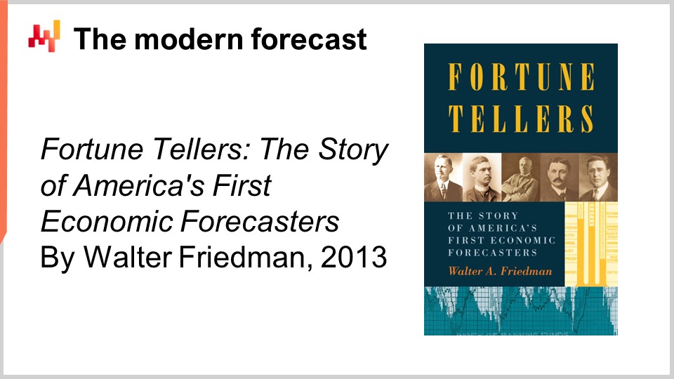
In order to understand the significance of probabilistic forecasts, a little bit of historical context is necessary. The modern form of forecasting, the statistical forecast, as opposed to divination, emerged at the very beginning of the 20th century. Forecasting emerged in a broader scientific context where hard sciences, a select few very successful disciplines like kinetics, electromagnetism, and chemistry, were able to achieve seemingly arbitrarily precise results. These results were obtained through essentially what amounted to a multi-century effort, which mould be traced back to, for example, Galileo Galilei, in developing superior technologies that would enable superior forms of measurements. More precise measurements, in turn, would fuel further scientific development by letting scientists test and challenge their theories and predictions in even more precise ways.
In this broader context where some sciences were incredibly successful, the emerging forecasting field at the very beginning of the 20th century took upon itself to essentially replicate what those hard sciences had accomplished in the realm of economics. For example, if we look at pioneers like Roger Babson, one of the fathers of modern economic forecasting, he established a successful economic forecasting company in the United States at the beginning of the 20th century. The motto of the company was quite literally, “For every action, there is an equal and opposite reaction.” Babson’s vision was to transpose the success of Newtonian physics into the realm of economics and ultimately to achieve equally precise results.
However, after more than a century of statistical academic forecasts, in which supply chains operate, the idea of achieving arbitrarily precise results, which translate in forecasting terms into achieving arbitrarily accurate forecasts, remains as elusive as it was more than a century ago. For a couple of decades, there have been voices in the broader supply chain world that have raised concerns that these forecasts are never going to become accurate enough. There has been a movement, such as lean manufacturing, that among others have been strong advocates for largely diminishing the reliance of supply chains on these unreliable forecasts. This is what just-in-time is about: if you can manufacture and serve just in time everything that the market needs, then suddenly you don’t need a reliable, accurate forecast anymore.
In this context, probabilistic forecasting is a rehabilitation of forecasting, but with much more modest ambitions. Probabilistic forecasting starts with the idea that there is an irreducible uncertainty about the future. All futures are possible, they are just not all equally possible, and the goal of probabilistic forecasting is to comparatively assess the respective likelihood of all those alternative futures, not to collapse all the possible futures into just one future.
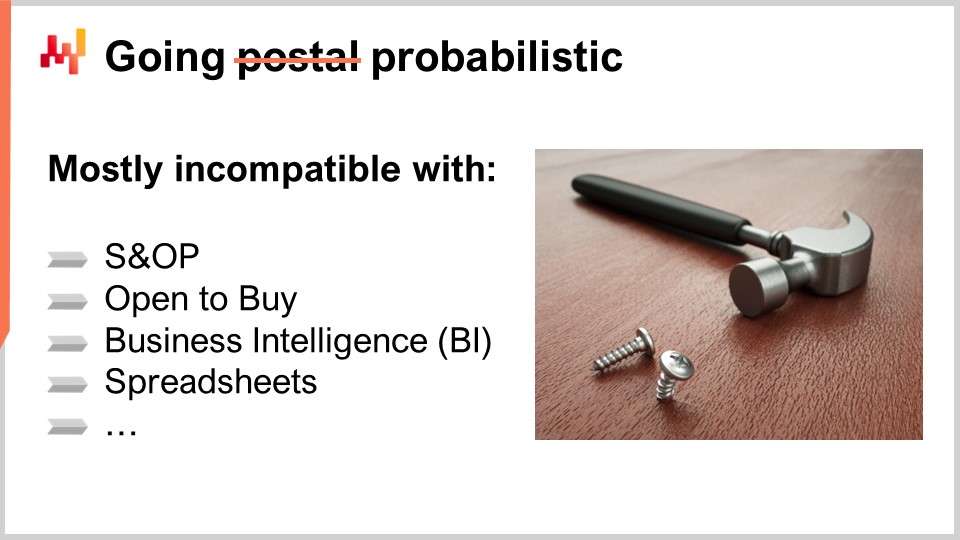
The Newtonian perspective on statistical economic forecasts has essentially failed. The opinion among our community that arbitrarily accurate forecasts can ever be achieved is largely gone. Yet, strangely enough, almost all supply chain software and a large amount of mainstream supply chain practices are actually rooted at their core on the assumption that such forecasts will ultimately be available.
For example, Sales and Operations Planning (S&OP) is rooted in the idea that a unified, quantified vision for the company can be achieved if all the stakeholders are put together and collaborate in constructing a forecast together. Similarly, open-to-buy is also essentially a method rooted in the idea that a top-down budgeting process, based on the idea that it is possible to construct arbitrarily precise top-down forecasts. Moreover, even when we look at many tools that are very common when it comes to forecasting and planning in the realm of supply chains, such as business intelligence and spreadsheets, those tools are extensively geared towards a point time-series forecast. Essentially, the idea is that you can have your historical data extended into the future, having one point per period of time of interest. These tools, by design, have an enormous amount of friction when it comes to even comprehending the sort of calculations that are involved with a probabilistic forecast, where there is not just one future but all possible futures.
Indeed, probabilistic forecasting is not about decorating a classic forecast with some kind of uncertainty. Probabilistic forecasting is also not about establishing a shortlist of scenarios, with each scenario being a classic forecast on its own. Mainstream supply chain methods typically don’t work with probabilistic forecasts because, at their core, they are implicitly or explicitly based on the idea that there exists some kind of reference forecast, and that everything will pivot around this reference forecast. In contrast, probabilistic forecasting is the frontal numerical assessment of all possible futures.
Naturally, we are limited by the amount of computing resources that we have, so when I say “all possible futures,” in practice, we will only look at a finite amount of futures. However, considering the sort of modern processing power that we have, the number of futures that we can actually consider ranges into the millions. That’s where business intelligence and spreadsheets struggle. They are not geared towards the sort of calculations that are involved when dealing with probabilistic forecasts. This is a problem of software design. You see, a spreadsheet has access to the very same computers and the very same processing power, but if the software doesn’t come with the right sort of design, then some tasks can be incredibly difficult to achieve, even if you have a vast amount of processing power.
Thus, from a supply chain perspective, the biggest challenge to adopt probabilistic forecasting is to let go of decades of tools and practices that are rooted in a very ambitious, but I believe misguided goal, namely that achieving arbitrarily accurate forecasts is possible. I would like to immediately point out that it would be incredibly misguided to think of probabilistic forecasting as a way to achieve more accurate forecasts. This is not the case. Probabilistic forecasts are not more accurate and they cannot be used as a drop-in replacement for classical, mainstream forecasts. The superiority of probabilistic forecasts lies in the ways that those forecasts can be exploited for supply chain purposes, especially decision-making purposes in the context of supply chains. However, our goal today is just to understand what those probabilistic forecasts are about, and the exploitation of those probabilistic forecasts will come in the next lecture.
This lecture is part of a series of supply chain lectures. I’m trying to keep those lectures quite independent from one another. However, we are reaching a point where it will really help the audience if those lectures are watched in sequence, as I will be frequently referencing what was presented in previous lectures.
So, this lecture is the third of the fifth chapter, which is dedicated to predictive modeling. In the very first chapter of this series, I presented my views on supply chains as both a field of study and a practice. In the second chapter, I presented methodologies. Indeed, most of the supply chain situations are adversarial in nature, and those situations tend to defeat naive methodologies. We need to have adequate methodologies if we want to achieve any degree of success in the realm of supply chains.
The third chapter was dedicated to supply chain parsimony, with an exclusive focus on the problem and the very nature of the challenge that we’re facing in various situations that supply chains cover. The idea behind supply chain parsimony is to ignore entirely all the aspects that are on the solution side, as we just want to be able to exclusively look at the problem before picking the solution that we want to use to address it.
In the fourth chapter, I surveyed a wide array of auxiliary sciences. These sciences are not supply chain per se; they are other fields of research that are adjacent or supportive. However, I believe that an entry-level command of those auxiliary sciences is a requirement for modern practice of supply chains.
Finally, in the fifth chapter, we delve into the techniques that let us quantify and assess the future, especially to produce statements about the future. Indeed, everything that we do in the supply chain reflects to some degree a certain anticipation of the future. If we can anticipate the future in a better way, then we will be able to make better decisions. That’s what this fifth chapter is about: getting quantifiably better insights about the future. In this chapter, probabilistic forecasts represent a pivotal way in our approach to tackle the future.
The rest of this lecture is divided into four sections of unequal length. First, we are going to review the most common types of forecasts, beyond the classic one. I will clarify what I mean by classic forecast in a moment. Indeed, too few people in supply chain circles realize that there are many options on the table. Probabilistic forecasting itself should be understood as an umbrella covering a fairly diverse set of tools and techniques.
Second, we will introduce metrics to assess the quality of probabilistic forecasts. No matter what happens, a well-designed probabilistic forecast will always tell you, “Well, there was a probability for this to happen.” So the question becomes: how do you sort out what is actually a good probabilistic forecast from a bad one? That’s where those metrics come into play. There are specialized metrics that are fully dedicated to the probabilistic forecasting situation.
Third, we will have an in-depth examination of one-dimensional distributions. They are the simplest sort of distribution, and while they have obvious limitations, they are also the easiest entry point into the realm of probabilistic forecasting.
Fourth, we will briefly touch on generators, which are frequently referred to as Monte Carlo methods. Indeed, there is a duality between generators and probability density estimators, and those Monte Carlo methods will give us a path to tackle higher-dimensional problems and forms of probabilistic forecasting.
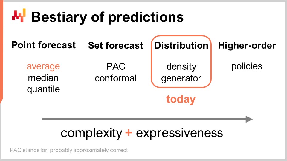
There are multiple types of forecasts, and this aspect should not be confused with the fact that there are multiple types of forecasting models. When models don’t belong to the same type or class of forecast, they are not even solving the same problems. The most common type of forecast is the point forecast. As an example, if I say that tomorrow the total sales in euros in a store will be 10,000 euros for the total sales aggregate of the day, I am making a point forecast about what will happen in this store tomorrow. If I repeat this exercise and start building a time series forecast by making a statement for the day of tomorrow, then another statement for the day after tomorrow, I will have multiple data points. However, all of that still remains a point forecast because, essentially, we are picking our battle by choosing a certain aggregation level and, at that aggregation level, our forecasts give us one single number, which is supposed to be the answer.
Now, within the type of point forecast, there are multiple subtypes of forecasts depending on which metric is being optimized. The most commonly used metric is probably the squared error, so we have a mean squared error, which gives you the average forecast. By the way, this tends to be the most commonly used forecast because it’s the only forecast that is at least somewhat additive. No forecast is ever fully additive; it always comes with tons of caveats. However, some forecasts are more additive than others, and clearly, average forecasts tend to be the most additive of the lot. If you want to have an average forecast, what you have is essentially a point forecast that is optimized against the mean squared error. If you use another metric, like the absolute error, and optimize against that, what you’re going to get is a median forecast. If you use the pinball loss function that we introduced in the very first lecture of this fifth chapter in this series of supply chain lectures, what you will get is a quantile forecast. By the way, as we can see today, I am classifying quantile forecasts as just another type of point forecast. Indeed, with the quantile forecast, you essentially get a single estimate. This estimate might come with a bias, which is intended. This is what quantiles are about, but nonetheless, in my view, it fully qualifies as a point forecast because the form of the forecast is just a single point.
Now, there is the set forecast, which returns a set of points instead of a single point. There is a variation depending on how you build the set. If we look at a PAC forecast, PAC stands for Probably Approximately Correct. This is essentially a framework introduced by Valiant about two decades ago, and it states that the set, which is your prediction, has a certain probability so that an outcome will be observed within your set that you’re predicting with a certain probability. The set that you produce is actually all the points that fall within a region characterized by a maximal distance to a point of reference. In a way, the PAC perspective on forecasting is already a set forecast because the output is not a point anymore. However, what we have is still a point of reference, a central outcome, and what we have is a maximal distance to this central point. We are just saying that there is a certain specified probability that the outcome will ultimately be observed to be within our prediction set.
The PAC approach can be generalized through the conformal approach. Conformal prediction states, “Here is a set, and I tell you that there is this given probability that the outcome will be within this set.” Where conformal prediction generalizes the PAC approach is that conformal predictions are not attached anymore to having a point of reference and the distance to the point of reference. You can shape this set any way you want, and you will still be part of the set forecast paradigm.
The future can be represented in an even more granular and complex way: the distribution forecast. The distribution forecast gives you a function that maps all the possible outcomes to their respective local probability densities. In a way, we start with the point forecast, where the forecast is just a point. Then we move to the set forecast, where the forecast is a set of points. Finally, the distribution forecast is technically a function or something that generalizes a function. By the way, when I use the term “distribution” in this lecture, it will always refer implicitly to a distribution of probabilities. Distribution forecasts represent something even richer and more complex than a set, and this will be our focus today.
There are two common ways to approach distributions: the density approach and the generator approach. When I say “density,” it basically refers to the local estimation of probability densities. The generator approach involves a Monte Carlo generative process that generates outcomes, called deviates, which are supposed to reflect the same local probability density. These are the two main ways to tackle distribution forecasts.
Beyond distribution, we have higher-order constructs. This might be a bit complicated to understand, but my point here, even though we are not going to cover higher-order constructs today, is just to outline that probabilistic forecasting, when focused on generating distributions, is not the end game; it’s just a step, and there is more. Higher-order constructs are important if we want to ever be able to achieve satisfying answers to simple situations.
To understand what higher-order constructs are about, let’s consider a simple retail store with a discount policy in place for products nearing their expiration dates. Obviously, the store doesn’t want to have dead inventory on their hands, so an automatic discount kicks in when products are very near their expiration dates. The demand this store would generate is highly dependent on this policy. Thus, the forecast we would like to have, which can be a distribution representing the probabilities for all possible outcomes, should be dependent on this policy. However, this policy is a mathematical object; it is a function. What we would like to have is not a probabilistic forecast but something more meta – a higher-order construct that, given a policy, can generate the resulting distribution.
From a supply chain perspective, when we move from one type of forecast to the next, we gain a lot more information. This is not to be confused with making the forecast more accurate; it is about gaining access to a different kind of information altogether, like seeing the world in black and white and suddenly gaining the ability to see colors instead of just gaining extra resolution. In terms of tooling, spreadsheets and business intelligence tools are somewhat adequate for dealing with point forecasts. Depending on the type of set forecast you’re considering, they may be adequate, but you’re already stretching their design capabilities. They are not really designed to deal with any kind of fancy set forecast beyond the obvious one, where you’re just defining a range with minimum and maximum values in the range of expected values. We will see that, essentially, if we want to have any chance of working with distribution forecasts or even higher-order constructs, we need a different kind of tooling altogether, although this should become clearer in a moment.
To get started with probabilistic forecasts, let’s try to characterize what makes a good probabilistic forecast. Indeed, no matter what happens, a probabilistic forecast will tell you that, no matter what sort of outcome you happen to observe, there was a probability for this thing to happen. So, under those conditions, how do you differentiate a good probabilistic forecast from a bad one? It’s certainly not because it’s probabilistic that suddenly all the forecasting models are good.
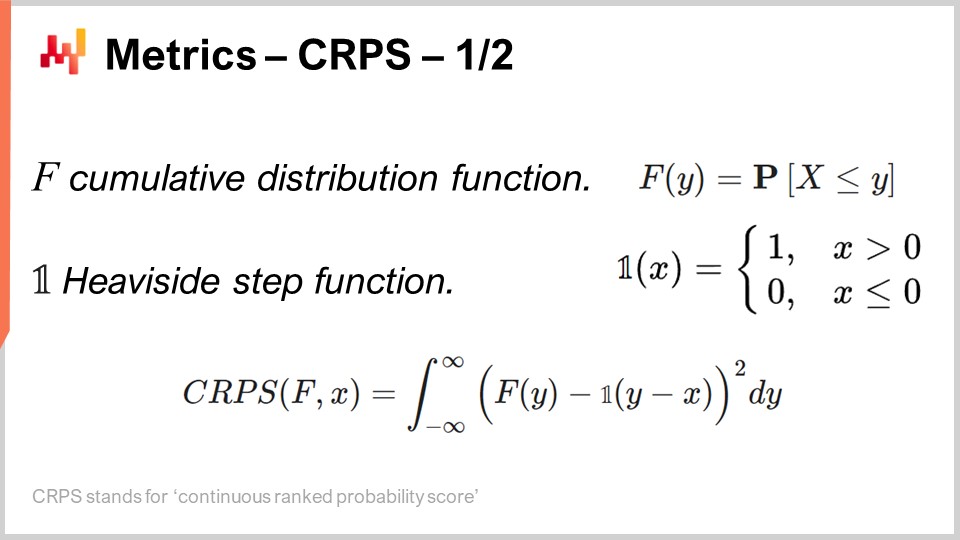
This is exactly what metrics dedicated to probabilistic forecasting are about, and the Continuous Ranked Probability Score (CRPS) is the generalization of the absolute error for one-dimensional probabilistic forecasts. I am absolutely sorry for this horrendous name – the CRPS. I didn’t come up with this terminology; it was handed over to me. The CRPS formula is given on the screen. Essentially, the function F is the cumulative distribution function; it is the probabilistic forecast being made. The point x is the actual observation, and the CRPS value is something that you compute between your probabilistic forecast and the one observation that you’ve just made.
We can see that, essentially, the point is turned into a quasi-probabilistic forecast of its own via the Heaviside step function. Introducing the Heaviside step function is just the equivalent of turning the point that we have just observed into a Dirac probability distribution, which is a distribution that concentrates all the probability mass on a single outcome. Then we have an integral, and essentially, the CRPS is doing some kind of shape matching. We are matching the shape of the CDF (cumulative distribution function) with the shape of another CDF, the one associated with the Dirac that matches the point that we observed.
From a point forecast perspective, the CRPS is puzzling not only because of the complicated formula but also because this metric takes two arguments that don’t have the same type. One of those arguments is a distribution, and the other one is just a single data point. So, we have an asymmetry here that does not exist with most other point forecast metrics, such as the absolute error and the mean squared error. In the CRPS, we are essentially comparing a point with a distribution.
If we want to understand more about what we compute with the CRPS, one interesting observation is that the CRPS has the same unit as the observation. For example, if x is expressed in euros, and the CRPS value between F and x is also homogeneous in terms of units to euros, that’s why I say that CRPS is a generalization of the absolute error. By the way, if you collapse your probabilistic forecast into a Dirac, the CRPS gives you a value that is exactly the absolute error.
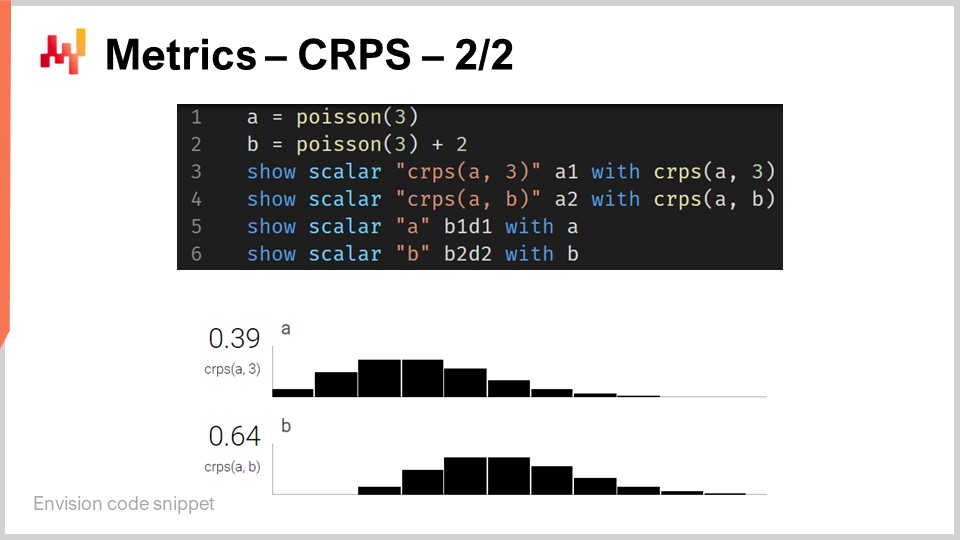
While the CRPS may seem quite intimidating and complicated, the implementation is actually reasonably straightforward. On the screen is a small Envision script that illustrates how the CRPS can be used from a programming language perspective. Envision is a domain-specific programming language dedicated to the predictive optimization of supply chains, developed by Lokad. In these lectures, I’m using Envision for the sake of clarity and concision. However, please note that there is nothing unique about Envision; the same results could be obtained in any programming language, be it Python, Java, JavaScript, C#, F#, or any other. My point is that it would just take more lines of code, so I’m sticking with Envision. All the code snippets given here in this lecture and, by the way, in the previous ones as well, are standalone and complete. You could technically copy and paste this code, and it would run. There are no modules involved, no hidden code, and no environment to be set up.
So, back to the code snippet. At lines one and two, we define one-dimensional distributions. I will be getting back to how those one-dimensional distributions actually work in Envision, but we have two distributions here: one is a Poisson distribution, which is a one-dimensional discrete distribution, and the second one on line two is the same Poisson distribution but shifted two units to the right. That’s what the “+2” stands for. At line three, we compute the CRPS distance between a distribution and the value 3, which is a number. So here, we are finding this asymmetry in terms of data types that I was talking about. Then, the results get displayed at the bottom, as you can see at the bottom of the screen.
At line four, we compute the CRPS between distribution A and distribution B. Although the classical definition of CRPS is between a distribution and a single point, it is completely straightforward to generalize this definition to a pair of distributions. All you have to do is to take the very same formula for CRPS and replace the Heaviside step function with the cumulative distribution function of the second distribution. The “show” statements from lines three to six result in the display that you can see at the bottom of the screen, which is literally a screenshot.
So, we see that using CRPS is not more difficult or complicated than using any special function, like the cosine function. Obviously, it is a bit of a pain if you have to re-implement the cosine yourself, but everything considered, there is nothing especially complicated about CRPS. Now, let’s move on.
The Monge-Kantorovich problem gives us insight into how to approach the shape-matching process at play in CRPS but with higher dimensions. Remember, CRPS is actually stuck with dimension one. Shape matching is conceptually something that could be generalized to any number of dimensions, and the Monge-Kantorovich problem is very interesting, doubly so because, at its core, it is actually a supply chain problem.
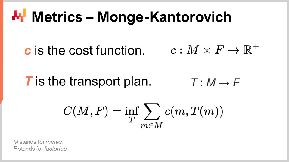
The Monge-Kantorovich problem, originally unrelated to probabilistic forecasting, was introduced by French scientist Gaspard Monge in a 1781 memoir titled “Mémoire sur la théorie des déblais et des remblais,” which could be roughly translated to “Memoir on the Theory of Moving Earth Around.” One way to understand the Monge-Kantorovich problem is to think of a situation where we have a list of mines, denoted as M on the screen, and a list of factories denoted as F. The mines produce ore, and the factories consume ore. What we want is to construct a transportation plan, T, that maps all the ore produced by the mines to the consumption required by the factories.
Monge defined capital C as the cost to move all the ore from the mines to the factories. The cost is the sum to transport all the ore from every mine to every factory, but there are obviously very inefficient ways to transport the ore. So, when we say we have a specific cost, we mean the cost reflects the optimal transportation plan. This capital C represents the best cost achievable by considering the optimal transportation plan.
This is essentially a supply chain problem that has been extensively studied over the centuries. In the complete problem formulation, there are constraints on T. For the sake of concision, I did not put all the constraints on the screen. There is a constraint, for example, that the transportation plan should not exceed the production capacity of every mine, and every factory should be fully satisfied, having an allocation that matches its requirements. There are plenty of constraints, but they are quite verbose, so I did not include them on the screen.
Now, while the transportation problem is interesting on its own, if we start interpreting the list of mines and the list of factories as two probability distributions, we have a way to turn a pointwise metric into a distribution-wise metric. This is a key insight about shape matching in higher dimensions through the Monge-Kantorovich perspective. Another term for this perspective is the Wasserstein metric, although it mostly concerns the non-discrete case, which is of lesser interest to us.
The Monge-Kantorovich perspective allows us to transform a pointwise metric, which can compute the difference between two numbers or two vectors of numbers, into a metric that applies to probability distributions operating over the same space. This is a very powerful mechanism. However, the Monge-Kantorovich problem is difficult to solve and requires substantial processing power. For the rest of the lecture, I will stick to techniques that are more straightforward to implement and execute.
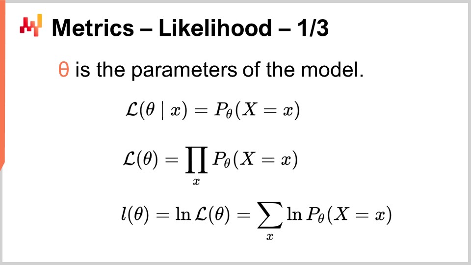
The Bayesian perspective consists of looking at a series of observations from the vantage point of a prior belief. The Bayesian perspective is usually understood in opposition to the frequentist perspective, which estimates the frequency of outcomes based on actual observations. The idea is that the frequentist perspective doesn’t come with prior beliefs. Thus, the Bayesian perspective gives us a tool known as the likelihood to assess the degree of surprise when considering the observations and a given model. The model, which is essentially a probabilistic forecasting model, is the formalization of our prior beliefs. The Bayesian perspective gives us a way to assess a dataset with regard to a probabilistic forecasting model. To understand how this is done, we should start with the likelihood for a single data point. The likelihood, when we have an observation x, is the probability to observe x according to the model. Here, the model is assumed to be fully characterized by theta, the parameters of the model. The Bayesian perspective typically assumes that the model has some kind of parametric form, and theta is the complete vector of all the model parameters.
When we say theta, we implicitly assume that we have a complete characterization of the probabilistic model, which gives us a local probability density for all the points. Thus, the likelihood is the probability to observe this one data point. When we have the likelihood for the model theta, it is the joint probability to observe all the data points in the dataset. We assume these points to be independent, so the likelihood is a product of probabilities.
If we have thousands of observations, the likelihood, as a product of thousands of values smaller than one, is likely to be numerically vanishingly small. A vanishingly small value is typically difficult to represent with the way floating point numbers are represented in computers. Instead of working with the likelihood directly, which is a vanishingly small number, we tend to work with the log likelihood. The log likelihood is just the logarithm of the likelihood, which has the incredible property of turning multiplication into addition.
The log likelihood of the model theta is the sum of the log of all the individual likelihoods for all the data points, as shown in the final equation line on the screen. The likelihood is a metric that gives us a goodness of fit for a given probabilistic forecast. It tells us how likely it is that the model generated the dataset we end up observing. If we have two probabilistic forecasts in competition, and if we put aside all other fitting issues for a moment, we should choose the model that gives us the highest likelihood or the highest log likelihood, because the higher the better.
The likelihood is very interesting because it can operate in high dimensions without complications, unlike the Monge-Kantorovich method. As long as we have a model that gives us a local probability density, we can use the likelihood, or more realistically, the log likelihood as a metric.
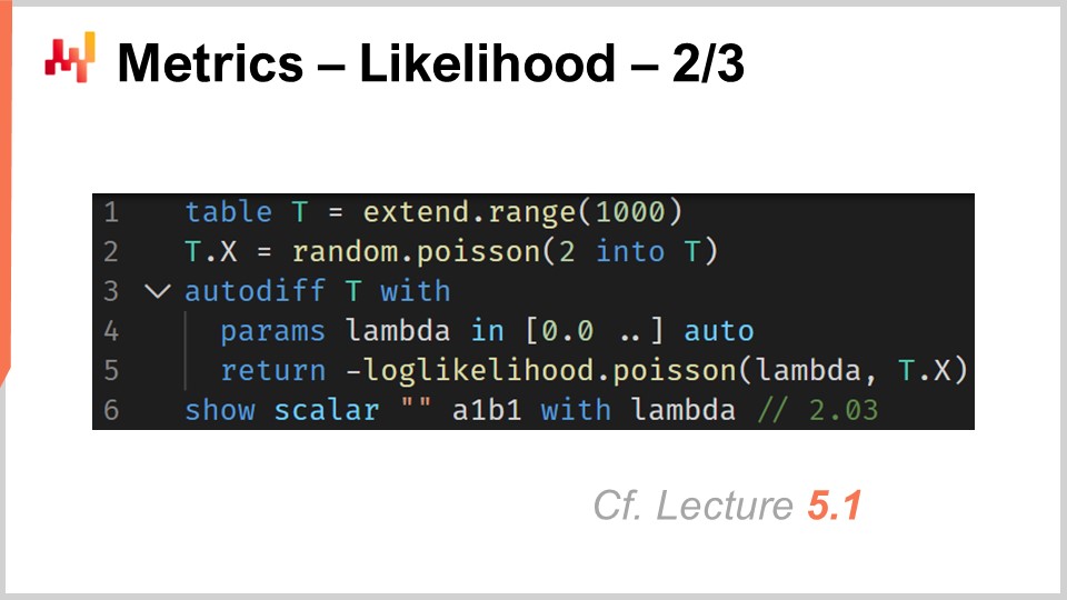
Furthermore, as soon as we have a metric that can represent the goodness of fit, it means we can optimize against this very metric. All it takes is a model with at least one degree of freedom, which basically means at least one parameter. If we optimize this model against the likelihood, our metric for goodness of fit, we will hopefully gain a trained model where we have learned to produce at least a decent probabilistic forecast. This is exactly what is being done here on the screen.
At lines one and two, we generate a mock dataset. We create a table with 2,000 lines, and then at line two, we generate 2,000 deviates, our observations from a Poisson distribution with a mean of two. So, we have our 2,000 observations. At line three, we start an autodiff block, which is part of the differentiable programming paradigm. This block will run a stochastic gradient descent and iterate many times over all the observations in the observation table. Here, the observation table is table T.
At line four, we declare the one parameter of the model, called lambda. We specify that this parameter should be exclusively positive. This parameter is what we will try to rediscover through the stochastic gradient descent. At line five, we define the loss function, which is just minus the log likelihood. We want to maximize the likelihood, but the autodiff block is trying to minimize the loss. Thus, if we want to maximize the log likelihood, we have to add this minus sign in front of the log likelihood, which is exactly what we have done.
The learned lambda parameter is put on display at line six. Unsurprisingly, the value found is very close to the value two, because we started with a Poisson distribution with a mean of two. We created a probabilistic forecasting model that is also parametric and of the same form, a Poisson distribution. We wanted to rediscover the one parameter of the Poisson distribution, and that is exactly what we get. We obtain a model that is within about one percent of the original estimate.
We have just learned our first probabilistic forecasting model, and all it took was essentially three lines of code. This is obviously a very simple model; nevertheless, it shows that there is nothing intrinsically complicated about probabilistic forecasting. It is not your usual mean square forecast, but aside from that, with the proper tools like differentiable programming, it is not more complicated than a classical point forecast.
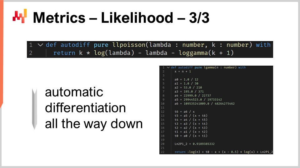
The log_likelihood.poisson function that we used previously is part of the standard library of Envision. However, there is no magic involved. Let’s have a look at how this function is actually implemented under the hood. The first two lines at the top give us the implementation of the log likelihood of the Poisson distribution. A Poisson distribution is fully characterized by its one parameter, lambda, and the log likelihood function only takes two arguments: the one parameter that fully characterizes the Poisson distribution and the actual observation. The actual formula I’ve written is literally textbook material. It’s what you get when you implement the textbook formula that characterizes the Poisson distribution. There is nothing fancy here.
Pay attention to the fact that this function is marked with the autodiff keyword. As we’ve seen in the previous lecture, the autodiff keyword ensures that automatic differentiation can flow correctly through this function. The log likelihood of the Poisson distribution is also using another special function, log_gamma. The log_gamma function is the logarithm of the gamma function, which is the generalization of the factorial function to complex numbers. Here, we only need the generalization of the factorial function to real positive numbers.
The implementation of the log_gamma function is slightly verbose, but it is again textbook material. It uses a continuous fraction approximation for the log_gamma function. The beauty here is that we have automatic differentiation working for us all the way down. We start with the autodiff block, calling the log_likelihood.poisson function, which is implemented as an autodiff function. This function, in turn, calls the log_gamma function, also implemented with the autodiff marker. Essentially, we are able to produce our probabilistic forecasting methods in three lines of code because we have a well-engineered standard library that has been implemented, paying attention to automatic differentiation.
Now, let’s move to the special case of one-dimensional discrete distributions. These distributions are all over the place in a supply chain and represent our entry point into probabilistic forecasting. For example, if we want to forecast lead times with daily granularity, we can say that there is a certain probability of having a one-day lead time, another probability of having a two-day lead time, three days, and so on. All of that builds up into a histogram of probabilities for lead times. Similarly, if we are looking at the demand for a given SKU on a given day, we can say that there is a probability of observing zero units of demand, one unit of demand, two units of demand, and so on.
If we pack all these probabilities together, we get a histogram representing them. Similarly, if we are thinking about the stock level of a SKU, we might be interested in assessing how much stock will be left for this given SKU at the end of the season. We can use a probabilistic forecast to determine the probability that we have zero units left in stock at the end of the season, one unit left in stock, two units, and so on. All of these situations fit the pattern of being represented through a histogram with buckets associated with every single discrete outcome of the phenomenon of interest.
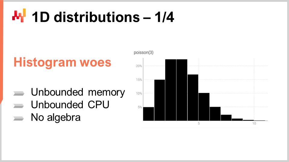
The histogram is the canonical way to represent a one-dimensional discrete distribution. Each bucket is associated with the mass of probability for the discrete outcome. However, putting aside the data visualization use case, histograms are a little underwhelming. Indeed, operating over histograms is a bit of a struggle if we want to do anything but visualizing those probability distributions. We have essentially two classes of problems with histograms: the first struggle is related to computing resources, and the second class of struggle is related to the programming expressiveness of histograms.
In terms of computing resources, we should consider that the amount of memory needed by a histogram is fundamentally unbounded. You can think of a histogram as an array that grows as large as needed. When dealing with a single histogram, even an exceptionally large one from a supply chain perspective, the amount of memory needed is a non-issue for a modern computer. The problem arises when you have not just one histogram, but millions of histograms for millions of SKUs in a supply chain context. If each histogram can grow fairly large, managing these histograms can become a challenge, especially considering that modern computers tend to offer non-uniform memory access.
Conversely, the amount of CPU needed to process these histograms is also unbounded. While the operations on histograms are mostly linear, processing time increases as the amount of memory grows due to non-uniform memory access. As a result, there is significant interest in putting strict boundaries on the amount of memory and CPU required.
The second struggle with histograms is the lack of an attached algebra. While you can perform bucket-wise addition or multiplication of values when considering two histograms, doing so will not result in something that makes sense when interpreting the histogram as a representation of a random variable. For example, if you take two histograms and perform point-wise multiplication, you end up with a histogram that does not even have a mass of one. This is not a valid operation from the perspective of an algebra of random variables. You can’t really add or multiply histograms, so you are limited in what you can do with them.
At Lokad, the approach we have found most practical to deal with these ubiquitous discrete one-dimensional distributions is to introduce a dedicated data type. The audience is probably familiar with common data types that exist in most programming languages, such as integers, floating point numbers, and strings. These are the typical primitive data types found everywhere. However, nothing prevents you from introducing more specialized data types that are especially fitting for our requirements from a supply chain perspective. This is exactly what Lokad did with the ranvar data type.
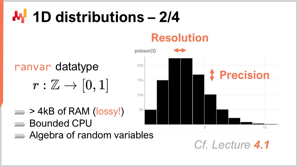
The ranvar data type is dedicated to one-dimensional discrete distributions, and the name is a shorthand for random variable. Technically, from a formal perspective, the ranvar is a function from Z (the set of all integers, positive and negative) to probabilities, which are numbers between zero and one. The total mass of Z is always equal to one, as it represents probability distributions.
From a purely mathematical perspective, some might argue that the amount of information that can be pushed into such a function can get arbitrarily large. This is true; however, the reality is that, from a supply chain perspective, there is a very clear limit to how much relevant information can be contained within a single ranvar. While it is theoretically possible to come up with a probability distribution that would require megabytes to represent, no such distribution exists that are relevant for supply chain purposes.
It is possible to engineer an upper bound of 4 kilobytes for the ranvar data type. By having a limit on the memory that this ranvar can take, we also end up with an upper bound CPU-wise for all operations, which is very important. Instead of having a naïve limit capping the buckets at 1,000, Lokad introduces a compression scheme with the ranvar data type. This compression is essentially a lossy representation of the original data, losing resolution and precision. However, the idea is to engineer a compression scheme that provides a sufficiently precise representation of the histograms, so that the degree of approximation introduced is negligible from a supply chain perspective.
The fine print of the compression algorithm involved with the ranvar data type is beyond the scope of this lecture. However, this is a very simple compression algorithm that is orders of magnitude simpler than the sorts of compression algorithms used for images on your computer. As a side benefit of having a limit on the memory that this ranvar can take, we also end up with an upper bound CPU-wise for all operations, which is very important. Finally, with the ranvar data type, the most important point is that we get an algebra of variables that give us a way to actually operate over these data types and do all the sort of things that we want to do with primitive data types, which is to have all sorts of primitives to combine them in ways that are fitting our requirements.
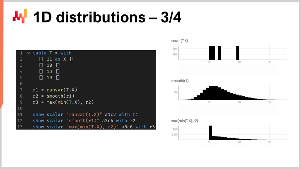
To illustrate what it means to work with ranvars, let’s consider a lead time forecasting situation, more specifically, a probabilistic forecasting of a lead time. On the screen is a short Envision script that shows how to build such a probabilistic forecast. At lines 1-5, we introduce the table T that contains the four lead times of variation, with values of 11 days, 10 days, 13 days, and 90 days. While four observations are very few, it is unfortunately very common to have very limited data points as far as lead time observations are concerned. Indeed, if we are considering an overseas supplier that gets two purchase orders per year, then it takes two years to collect those four data points. Thus, it is important to have techniques that can operate even with an incredibly limited set of observations.
At line 7, we create a ranvar by directly aggregating the four observations. Here, the term “ranvar” that appears on line 7 is actually an aggregator that takes a series of numbers as inputs and returns a single value of the ranvar data type. The result is displayed on the top right of the screen, which is an empirical ranvar.
However, this empirical ranvar is not a realistic depiction of the actual distribution. For example, while we can observe a lead time of 11 days and a lead time of 13 days, it feels unrealistic to not be able to observe a lead time of 12 days. If we interpret this ranvar as a probabilistic forecast, it would say that the probability of ever observing a lead time of 12 days is zero, which seems incorrect. This is obviously an overfitting problem.
To remedy this situation, at line 8, we smooth the original ranvar by calling the function “smooth.” The smooth function essentially replaces the original ranvar with a mixture of distributions. For every bucket of the original distribution, we replace the bucket with a Poisson distribution of a mean centered on the bucket, weighted according to the respective probability of the buckets. Through the smooth distribution, we get the histogram that is displayed in the middle on the right of the screen. This is already looking much better; we don’t have any bizarre gaps anymore, and we don’t have a zero probability in the middle. Moreover, when looking at the probability of observing a 12-day lead time, this model gives us a non-zero probability, which sounds much more reasonable. It also gives us a non-zero probability to go beyond 20 days, and considering that we had four data points and already observed a lead time of 19 days, the idea that a lead time as high as 20 days is possible feels very reasonable. Thus, with this probabilistic forecast, we have a nice spread that represents a non-zero probability for those events, which is very good.
However, on the left, we have something a little strange. While it’s okay for this probability distribution to spread to the right, the same cannot be said about the left. If we consider that the lead times we observed were the results of transportation times, due to the fact that it takes nine days for the truck to arrive, it feels unlikely that we would ever observe a lead time of three days. In this regard, the model is quite unrealistic.
Thus, at line 9, we introduce a conditionally adjusted ranvar by saying that it must be larger than the smallest lead time ever observed. We have “min_of(T, x)” which takes the smallest value among the numbers of the table T, and then we use “max” to do the max between a distribution and a number. The result has to be bigger than this value. The adjusted ranvar is displayed on the right at the very bottom, and here we see our final lead time forecast. The last one feels like a very reasonable probabilistic forecast of the lead time, considering that we have an incredibly limited dataset with only four data points. We cannot say that it’s a great probabilistic forecast; however, I would argue that this is a production-grade forecast, and these sorts of techniques would work fine in production, unlike an average point forecast which would vastly underestimate the risk of varying lead times.
The beauty of probabilistic forecasts is that, while they can be very crude, they already give you some extent of mitigation potential for ill-informed decisions that would result from the naive application of an average forecast based on the observed data.
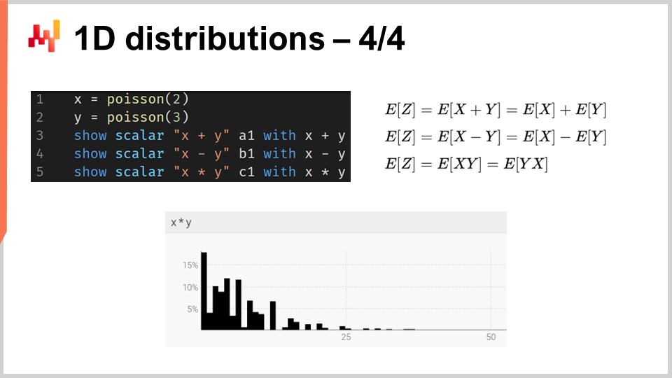
More generally, ranvars support a whole range of operations: it is possible to add, subtract, and multiply ranvars, just like it is possible to add, subtract, and multiply integers. Under the hood, because we are dealing with discrete random variables in terms of semantics, all these operations are implemented as convolutions. On the screen, the histogram displayed at the bottom is obtained via the multiplication of two Poisson distributions, respectively of mean two and three. In supply chain, the multiplication of random variables is called a direct convolution. In the context of supply chain, the multiplication of two random variables makes sense to represent, for example, the outcomes you can get when clients are seeking the same products but with varying multipliers. Let’s say we have a bookstore that serves two cohorts of clients. On one side, we have the first cohort consisting of students, who buy one unit when they walk into the store. In this illustrative bookstore, we have a second cohort comprised of professors, who buy 20 books when they enter the store.
From a modeling perspective, we could have one probabilistic forecast that represents the arrival rates in the bookstore of either students or professors. This would give us the probability of observing zero customers for the day, one customer, two customers, etc., revealing the probability distribution of observing a certain number of customers for any given day. The second variable would give you the respective probabilities of buying one (students) versus buying 20 (professors). To have a representation of the demand, we would just multiply those two random variables together, resulting in a seemingly erratic histogram that reflects the multipliers present in the consumption patterns of your cohorts.
Monte Carlo generators, or simply generators, represent an alternative approach to probabilistic forecasting. Instead of exhibiting a distribution that gives us the local probability density, we can exhibit a generator that, as the name suggests, generates outcomes expected to follow implicitly the very same local probability distributions. There is a duality between generators and probability densities, meaning that the two are essentially two facets of the same perspective.
If you have a generator, it is always possible to average out the outcomes obtained from this generator to reconstruct estimates of the local probability densities. Conversely, if you have local probability densities, it is always possible to draw deviates according to this distribution. Fundamentally, these two approaches are just different ways to look at the same probabilistic or stochastic nature of the phenomenon we are trying to model.
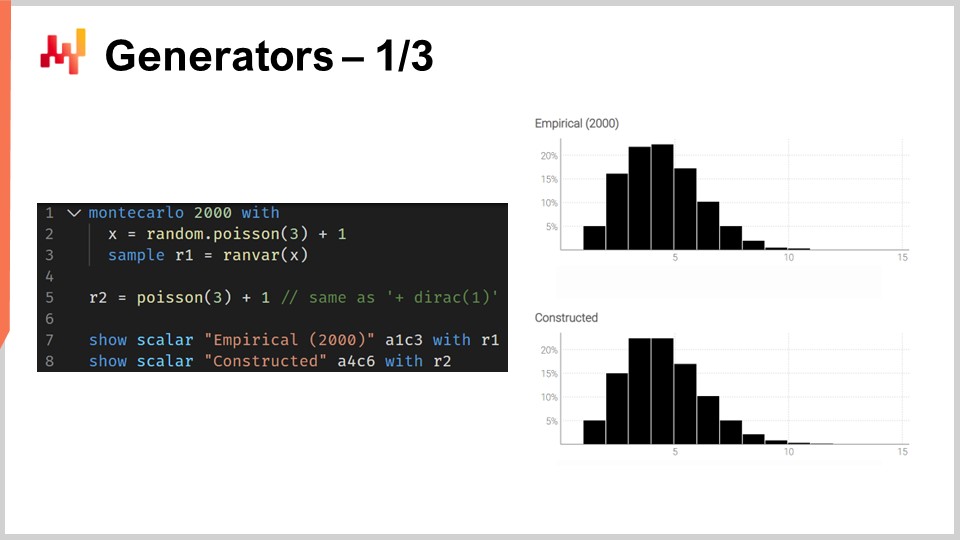
The script on the screen illustrates this duality. At line one, we introduce a Monte Carlo block, which will be iterated on by the system, just like the auto-differentiation blocks are iterated through many steps of stochastic gradient descent. The Monte Carlo block will be executed 2,000 times, and from this block, we will collect 2,000 deviates.
At line two, we draw a deviate from a Poisson distribution of mean three and then add one to the deviate. Essentially, we obtain a random number from this Poisson distribution and then add one. At line three, we collect this deviate into L1, which is acting as an accumulator for the aggregator ranvar. This is the exact same aggregator as the one we introduced previously for our lead time example. Here, we are collecting all those observations into L1, which gives us a one-dimensional distribution obtained through a Monte Carlo process. At line five, we construct the very same one-dimensional discrete distribution, but this time, we do it with the algebra of random variables. So, we just use Poisson minus three and add one. At line five, there is no Monte Carlo process going on; it is a pure matter of discrete probabilities and convolutions.
When we compare the two distributions visually at lines seven and eight, we see that they are almost identical. I say “almost” because, while we are using 2,000 iterations, which is a lot, it is not infinite. The deviations between the exact probabilities you get with ranvar and the approximate probabilities you get with the Monte Carlo process are still noticeable, though not large.
Generators are sometimes called simulators, but make no mistake, they are the same thing. Whenever you have a simulator, you have a generative process that implicitly underlies a probabilistic forecasting process. Whenever you have a simulator or generator involved, the question that should be on your mind is: what is the accuracy of this simulation? It is not accurate by design, just as it is very possible to have completely inaccurate forecasts, probabilistic or not. You can very easily get a completely inaccurate simulation.
With generators, we see that simulations are just one way to look at the probabilistic forecasting perspective, but this is more like a technical detail. It doesn’t change anything about the fact that, in the end, you want to have something that is an accurate depiction of the system you are trying to characterize with your forecast, probabilistic or not.
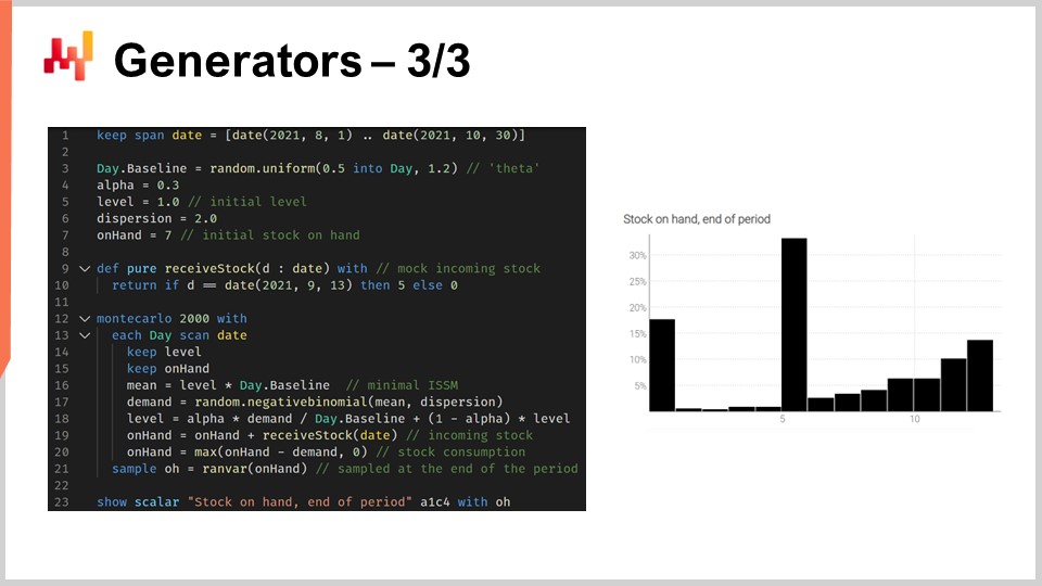
The generative approach is not only very useful, as we will see with a specific example in a minute, but it is also conceptually easier to grasp, at least slightly, compared to the approach with probability densities. However, the Monte Carlo approach is not without technicalities either. There are a few things that are necessary if you want to make this approach viable in a production context for an actual real-world supply chain.
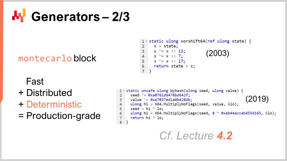
First, generators must be fast. Monte Carlo is always a trade-off between the number of iterations you would like to have and the number of iterations you can afford, considering the computing resources available. Yes, modern computers have plenty of processing power, but Monte Carlo processes can be incredibly resource-consuming. You want something that is, by default, super fast. If we go back to the ingredients introduced in the second lecture of the fourth chapter, we have very fast functions like ExhaustShift or WhiteHash that are essential to the construction of the primitives that let you generate elementary random generators that are super fast. You need that, otherwise, you’re going to struggle. Second, you need to distribute your execution. The naive implementation of a Monte Carlo program is just to have a loop that iterates sequentially. However, if you’re only using a single CPU to tackle your Monte Carlo requirements, essentially, you are getting back to the computing power that characterized computers two decades ago. This point was touched upon in the very first lecture of the fourth chapter. Over the last two decades, computers have become more powerful, but it was mostly by adding CPUs and degrees of parallelization. So, you need to have a distributed perspective for your generators.
Lastly, the execution must be deterministic. What does that mean? It means that if the same code is run twice, it should give you the exact same results. This might feel counterintuitive because we are dealing with randomized methods. Nevertheless, the need for determinism emerged very quickly. It has been discovered in a painful way during the ’90s when finance started using Monte Carlo generators for their pricing. Finance went down the path of probabilistic forecasting quite a while ago and made extensive use of Monte Carlo generators. One of the things they learned was that if you do not have determinism, it becomes nearly impossible to replicate the conditions that generated a bug or a crash. From a supply chain perspective, mistakes in purchase order calculations can be incredibly costly.
If you want to achieve some degree of production readiness for the software that governs your supply chain, you need to have this deterministic property whenever you’re dealing with Monte Carlo. Beware that many open-source solutions come from academia and do not care at all about production readiness. Make sure that when you’re dealing with Monte Carlo, your process is super fast by design, distributed by design, and deterministic, so that you have a chance to diagnose the bugs that will inevitably arise over time in your production setup.
We have seen a situation where a generator was introduced to replicate what was otherwise done with a ranvar. As a rule of thumb, whenever you can get away with just probability densities with random variables without involving Monte Carlo, it is better. You get more precise results, and you don’t have to worry about numerical stability that is always a bit tricky with Monte Carlo. However, the expressiveness of the algebra of random variables is limited, and that’s where Monte Carlo really shines. These generators are more expressive because they let you apprehend situations that cannot be tackled with just an algebra of random variables.
Let’s illustrate this with a supply chain situation. Consider a single SKU with an initial stock level, a probabilistic forecast for the demand, and a period of interest spanning over three months, with an incoming shipment in the middle of the period. We assume that the demand is either serviced immediately from the stock on hand or it is lost forever. We want to know the expected stock level at the end of the period for the SKU, as knowing that will help us decide how much risk we have in terms of dead inventory.
The situation is treacherous because it has been engineered in a way that there is a third chance for a stockout to happen right in the middle of the period. The naive approach would be to take the initial stock level, the distribution of demand for the entire period, and subtract the demand from the stock level, resulting in the remaining stock level. However, this does not take into account the fact that we might lose a fair portion of the demand if we have a stockout while the incoming replenishment is still pending. Doing it the naive way would underestimate the amount of stock we’ll have at the end of the period and overestimate the amount of demand that will be served.
The script on display models the occurrence of stockouts so that we can have a correct estimator for the stock level for this SKU at the end of the period. From lines 1 to 10, we are defining the mock data that characterizes our model. Lines 3 to 6 contain the parameters for the ISSM model. We have already seen the ICSM model in the very first lecture of this fifth chapter. Essentially, this model generates a demand trajectory with one data point per day. The period of interest is defined in the day table, and we have the parameters for this trajectory at the very beginning.
In the previous lectures, we introduced the AICSM model and the methods needed through differentiable programming to learn these parameters. Today, we are using the model, assuming that we have learned everything we need to learn. At line 7, we define the initial stock on hand, which would typically be obtained from the ERP or WMS. At lines 9 and 10, we define the quantity and the date for the replenishment. These data points would typically be obtained as an estimated time of arrival given by the supplier and stored in the ERP. We assume that the delivery date is perfectly known; however, it would be straightforward to replace this single date with a probabilistic forecast of the lead time.
From lines 12 to 21, we have the ISSM model that generates the demand trajectory. We are within a Monte Carlo loop, and for every Monte Carlo iteration, we iterate over every single day of the period of interest. The iteration of days starts at line 13. We have the ESSM mechanics going on, but at lines 19 and 20, we update the on-hand variable. The on-hand variable is not part of the ISSM model; this is something extra. At line 19, we say that the stock on hand is the stock on hand from yesterday plus the incoming shipment, which will be zero for most of the days and five units for September 13th. Then, on line 20, we update the stock on hand by saying that a certain number of units are consumed by the demand of the day, and we have this max 0 to say that the stock level cannot go into the negatives.
Finally, we collect the final stock on hand at line 21, and at line 23, this final stock on hand is put on display. This is the histogram that you see on the right of the screen. Here, we see a distribution with a very irregular shape. This shape cannot be obtained through the algebra of random variables. Generators are incredibly expressive; however, you should not confuse the expressiveness of these generators with accuracy. While generators are incredibly expressive, it is non-trivial to assess the accuracy of such generators. Make no mistake, every time you have a generator or simulator at play, you have a probability forecast at play, and simulations can be dramatically inaccurate, just like any forecast, probabilistic or otherwise.

It has been a long lecture already, and yet there are many topics I haven’t even touched on today. Decision-making, for example, if all futures are possible, how do we decide anything? I haven’t answered this question, but it will be addressed in the next lecture.
Higher dimensions are also important to consider. One-dimensional distribution is a starting point, but a supply chain needs more. For example, if we hit a stock-out for a given SKU, we may experience cannibalization, where customers naturally fall back to a substitute. We would like to model this, even if in a crude fashion.
High order constructs also play a role. As I said, forecasting demand is not like forecasting the movements of planets. We have self-prophetic effects all over the place. At some point, we want to consider and factor in our pricing policies and stock replenishment policies. To do that, we need higher order constructs, which means given a policy, you get a probabilistic forecast of the outcome, but you have to inject the policy inside the higher order constructs.
Moreover, mastering probabilistic forecasts involves numerous numerical recipes and domain expertise to know which distributions are most likely to fit certain situations nicely. In this series of lectures, we will introduce more examples later.
Finally, there is the challenge of change. Probabilistic forecasting is a radical departure from mainstream supply chain practices. Frequently, the technicalities involved with probabilistic forecasts are only a small part of the challenge. The difficult part is to reinvent the organization itself, so it can start using these probabilistic forecasts instead of relying on point forecasts, which are essentially wishful thinking. All these elements will be covered in later lectures, but it will take time as we have a lot of ground to cover.
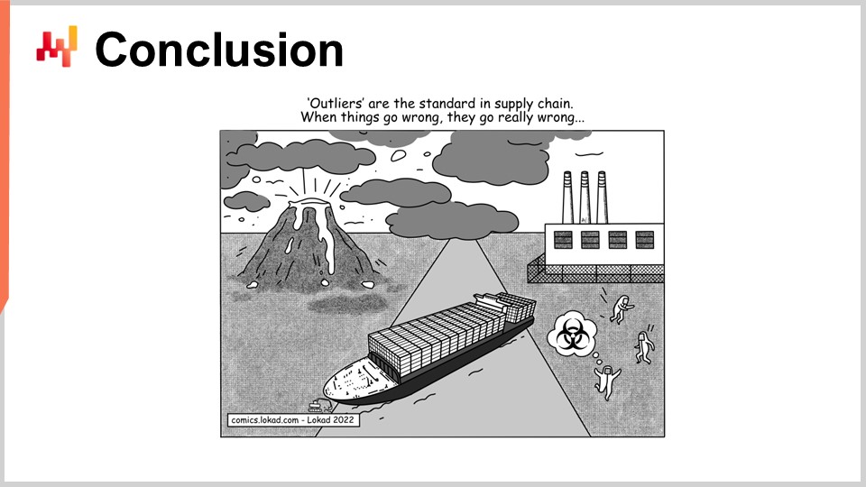
In conclusion, probabilistic forecasts represent a radical departure from the point forecast perspective, where we expect some kind of consensus on the one future that is supposed to come to pass. Probabilistic forecasting is based on the observation that the uncertainty of the future is irreducible. One century of forecasting science has demonstrated that all attempts at something that would even be close to accurate forecasts have failed. Thus, we are stuck with many indefinite futures. However, probabilistic forecasts give us techniques and tools to quantify and assess these futures. Probabilistic forecasting is a significant achievement. It took almost a century to come to terms with the idea that economic forecasting wasn’t like astronomy. While we can predict the exact position of a planet a century from now with great accuracy, we don’t have any hope of achieving anything remotely equivalent in the realm of supply chains. The idea of having one forecast to rule them all is just not coming back. Yet, many companies still cling to the hope that at some point, the one true accurate forecast will ever be achieved. After a century of attempts, this is essentially wishful thinking.
With modern computers, this one-future perspective is not the only perspective in town. We have alternatives. Probabilistic forecasting has been around since the 90s, so that’s three decades ago. At Lokad, we have been using probabilistic forecasting to drive supply chains in production for over a decade. It may not be mainstream yet, but it is very far from being science fiction. It has been a reality for many companies in finance for three decades and in the world of supply chain for one decade.
While probabilistic forecasts may seem intimidating and highly technical, with the right tooling, it is just a few lines of code. There is nothing particularly difficult or challenging about probabilistic forecasting, at least not compared to other types of forecasts. The biggest challenge when it comes to probabilistic forecasting is to give up the comfort associated with the illusion that the future is perfectly under control. The future is not perfectly under control and never will be, and all things considered, it is probably for the best.
This concludes this lecture for today. Next time, on the 6th of April, I will be presenting decision-making in retail inventory dispatch, and we’ll see how probabilistic forecasts that have been presented today can be put to good use to drive a basic supply chain decision, namely inventory replenishment in a retail network. The lecture will take place on the same day of the week, Wednesday, at the same time of the day, 3 PM, and it will be the first Wednesday of April.
Question: Can we optimize resolution on precision versus RAM volume for Envision?
Yes, absolutely, although not in Envision itself. This is a choice that we made in the design of Envision. My approach when it comes to supply chain scientists is to liberate them from low-level technicalities. Envision’s 4 kilobytes is a lot of space, allowing for an accurate depiction of your supply chain situation. So, the approximation you’re losing in terms of resolution and precision is inconsequential.
Certainly, when it comes to the design of your compression algorithm, there are plenty of trade-offs to be considered. For example, buckets that are very close to zero need to have a perfect resolution. If you want to have the probability of observing zero units of demand, you don’t want your approximation to lump together the buckets for zero demand, one unit, and two units. However, if you are looking at buckets for the probability of observing 1,000 units of demand, lumping together 1,000 and 1,001 units of demand is probably fine. So, there are plenty of tricks for developing a compression algorithm that really fits supply chain requirements. This is orders of magnitude simpler compared to what is going on for image compression. My take is that a correctly designed tooling would basically abstract the problem for supply chain scientists. This is too low level, and you don’t need to micro-optimize in most cases. If you’re Walmart and you have not just 1 million SKUs but several hundred million SKUs, then micro-optimizing might make sense. However, unless you’re talking about exceedingly large supply chains, I believe you can have something that is good enough so that the performance hit by not having complete optimization is mostly inconsequential.
Question: What are the practical considerations to be taken into account from a supply chain perspective while optimizing those parameters?
When it comes to probabilistic forecasting in supply chain, having a precision more than one out of 100,000 is typically inconsequential, just because you never have enough data to have an accuracy in terms of estimation of your probabilities that is more granular than one part out of 100,000.
Question: What industry benefits the most from the probabilistic forecasting approach?
The short answer is, the more erratic and irregular your patterns are, the bigger the benefits. If you have intermittent demand, you have big benefits; if you have erratic demand, you have big benefits; if you have widely varying lead times and erratic shocks in your supply chains, you benefit the most. At the other extreme end of the spectrum, let’s say, for example, if we were looking at the supply chain of water distribution, the consumption of water is extremely smooth and nearly never has any big shocks – only micro shocks at most. This is the sort of problem that does not benefit from the probabilistic approach. The idea is there are a few situations where classic point forecasts give you very accurate forecasts. If you’re in a situation where your forecasts for all your products have less than a five percent error when looking ahead, then you don’t need probabilistic forecasts; you are in a situation where having a really accurate forecast actually works. However, if you are like many companies in situations where your forecast accuracy is very low, with a 30% or more divergence, then you benefit from probabilistic forecasting greatly. By the way, when I say 30% forecasting error, I’m always referring to the very disaggregated forecast. Many companies will tell you their forecasts are 5% accurate, but if you aggregate everything, this can be a very misleading perception of your forecasting accuracy. Your forecasting accuracy only matters at the most disaggregated level, typically at the SKU level and the daily level, because your decisions are taken at the SKU level and daily level. If at the SKU level and daily level, you can get your most disaggregated forecasts within 5% accuracy, then you don’t need probabilistic forecasts. However, if you observe double-digit inaccuracies in terms of percentages, then you will benefit from probabilistic forecasting greatly.
Question: As lead times can be seasonal, would you decompose lead time forecasts into multiple ones, each one for each distinct season, to avoid looking at a multimodal distribution?
This is a good question. The idea here is that you would typically build a parametric model for your lead times that include a seasonality profile. Dealing with seasonality for lead times is not fundamentally very different from dealing with any other cyclicality, as we did in the previous lecture for demand. The typical way is not to build multiple models, because as you correctly pointed out, if you have multiple models, you will observe all sorts of bizarre jumps when you go from one modality to the next. It’s typically better to just have one model with a seasonality profile in the middle of the model. It would be like a parametric decomposition where you have a vector that gives you the weekly effect that impacts the lead time at a certain week of the year. Maybe we will have time in a later lecture to give a more extensive example of that.
Question: Is probabilistic forecasting a good approach when you want to forecast intermittent demand?
Absolutely. In fact, I believe that when you have intermittent demand, probabilistic forecasting is not only a good method, but the classical point forecast is just completely nonsensical. With the classical forecast, you would typically struggle dealing with all those zeros. What do you make of those zeros? You end up with a value that is very low and fractional, which doesn’t really make sense. With intermittent demand, the question that you really want to answer is: Is my stock large enough to service those spikes of demand that tend to arise once in a while? If you use an average forecast, you will never know that.
Just to get back to the bookstore example, if you say that in a given week you observe one unit of demand per day on average, how many books do you need to keep in your bookstore to have a high quality of service? Let’s assume that the bookstore is replenished every single day. If the only people you are serving are students, then if you have on average one unit of demand every single day, having three books in stock will result in a very high quality of service. However, if once in a while you have a professor who comes in and is looking for 20 books at once, then your quality of service, if you only have three books in the store, will be abysmal because you will never be able to serve any of the professors. This is typically the case with intermittent demand – it’s not just the fact that demand is intermittent, but also that some spikes of demand can vary significantly in terms of magnitude. That’s where probabilistic forecasting really shines, as it can capture the fine structure of the demand instead of just lumping it all together into averages where all this fine structure is lost.
Question: If we replace lead time with a distribution, will the spike represented by a smooth bell curve on the first slide for the generator?
To some extent, if you randomize more, you tend to spread things around. On the first slide about the generator, we would have to run the experiment with various settings to see what we get. The idea is that when we want to replace lead time with a distribution, we do so because we have an insight on the problem that tells us that lead time is varying. If we trust our supplier absolutely and they have been incredibly reliable, then it is perfectly fine to say that the ETA (estimated time of arrival) is what it is and is an almost perfect estimate of the real thing. However, if we have seen that in the past suppliers were sometimes erratic or missing the target, then it is better to replace the lead time with a distribution.
Introducing a distribution to replace lead time doesn’t necessarily smooth the outcomes that you get at the end; it depends on what you’re looking at. For example, if you’re looking at the most extreme case of overstock, a varying lead time may even exacerbate the risk of having dead inventory. Why is that? If you have a very seasonal product and a varying lead time, and the product arrives after the end of the season, you are left with a product that is out of season, which magnifies the risk of having dead inventory at the end of the season. So, it is tricky. The fact that you turn a variable into its probabilistic replacement will not naturally smooth what you will observe; sometimes, it can make the distribution even sharper. So, the answer is: it depends.
Excellent, I think that’s all for today. See you next time.
