00:00 Introduction
02:53 Decisions vs Artifacts
10:07 Experimental optimization
13:51 The story so far
17:01 Today’s decisions
19:36 The manifesto of the quantitative supply chain
21:01 The retail stock allocation problem
24:49 Economic forces on the store SKU
29:35 Reifying the futures
32:41 Reifying the options - 1/3
38:25 Reifying the options - 2/3
43:02 Reifying the options - 3/3
44:44 Stock reward function - 1/2
51:41 Stock reward function - 2/2
56:19 Prioritized stock allocations - 1/4
59:59 Prioritized stock allocations - 2/4
01:03:39 Prioritized stock allocations - 3/4
01:06:34 Prioritized stock allocations - 4/4
01:12:58 Smoothing the warehouse flow - 1/2
01:16:48 Smoothing the warehouse flow - 2/2
01:22:12 Action reward function
01:25:02 The real world is messy
01:27:38 Conclusion
01:30:00 Upcoming lecture and audience questions
Description
Supply chain decisions require risk-adjusted economic assessments. Converting probabilistic forecasts into economic assessments is nontrivial and require dedicated tooling. However, the resulting economic prioritization, illustrated by stock allocations, proves itself more powerful than traditional techniques. We start with the retail stock allocation challenge. In a 2-echelon network that includes both a distribution center (DC) and multiple stores, we need to decide how to allocate the stock of the DC to the stores, knowing that all stores compete for the same stock.
Full transcript
Welcome to this series of supply chain lectures. I’m Joannes Vermorel, and today I will be presenting “Retail Stock Allocation with Probabilistic Forecasts.” Retail stock allocation is a simple yet fundamental challenge: when and how much stock do you decide to move at any point in time between the distribution centers and the stores you operate? The decision to move stock depends on future demand, thus a demand forecast of some kind is needed.
However, retail demand at the store level is uncertain, and the uncertainty of future demand is irreducible. We need a forecast that properly reflects this irreducible uncertainty of the future, thus a probabilistic forecast is needed. Yet, making the most of probabilistic forecasts in order to optimize supply chain decisions is a non-trivial task. It would be tempting to recycle an existing inventory technique that has been originally designed with a classic deterministic forecast in mind. However, doing so would defeat the very reason why we introduced probabilistic forecasts in the first place.
The goal of this lecture is to learn how to make the most of probabilistic forecasts in their native form to optimize supply chain decisions. As a first example, we will be considering the retail stock allocation problem, and through the examination of this problem, we will see how we can actually optimize the stock level at the store level. Additionally, through the examination of probabilistic forecasts, we can even address new classes of supply chain problems, such as smoothing the flow of inventory from the distribution centers to the stores in order to optimize and reduce the operating cost of the network.
This lecture opens the sixth chapter of this series, which is dedicated to decision-making techniques and processes in a supply chain context. We will see that decisions must be optimized with the entire supply chain network in mind, as an integrated system, as opposed to performing a series of isolated local optimizations. For example, taking a narrow perspective of the SKU (stock-keeping unit).
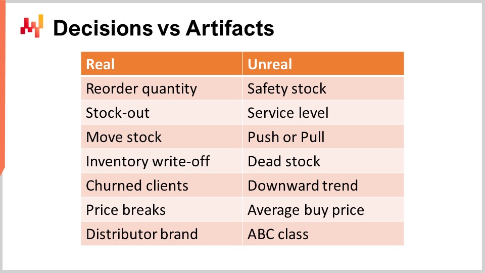
The first step to tackle supply chain decisions is to identify actual supply chain decisions. A supply chain decision has a direct, physical, tangible impact on the supply chain. For example, moving one unit of stock from the distribution center to a store is real; as soon as you do that, there is one extra unit on the shelves of the store and there is one unit that is now missing from the distribution center and that cannot be reallocated anywhere else.
On the contrary, an artifact has no direct physical tangible impact on the supply chain. An artifact is typically either an intermediate calculation step that ultimately leads to a supply chain decision, or it is a statistical estimate of some kind that characterizes a property of a part of your supply chain system. Unfortunately, I can’t help but observe a great deal of confusion in the supply chain literature when it comes to distinguishing decisions from artifacts.
Beware, returns on investments are exclusively obtained through the improvement of decisions. Improving artifacts is almost always inconsequential, and that is at best. At worst, if a company spends too much time improving artifacts, this becomes a distraction that prevents the company from improving its actual supply chain decisions. On the screen is a list of confusions that I frequently observe in mainstream supply chain circles.
For example, let’s start with safety stock. This stock is not real; you don’t have two stocks, the safety stock and the working stock. There is only one stock, and the only decision that can be taken is whether more is needed or not. Reordering a quantity is real, but safety stock is not. Similarly, the service level isn’t real either. The service level is very much model dependent. Indeed, in retail demand, sales data are sparse. Thus, if you take any given SKU, you typically have too little data to compute a meaningful service level by just inspecting the SKU. The way you approach service level is through modeling techniques and statistical estimates, which are fine, but again, this is an artifact, not reality. This is literally a mathematical perspective that you have on your supply chain.
Similarly, push or pull is also a matter of perspective. A proper numerical recipe that operates, taking into account the whole supply chain network, is only going to consider the opportunity of moving one unit of stock from one origin toward a destination. What is real is the stock movement; what is just a matter of perspective is whether you want to trigger this stock movement based on conditions related to the origin or the destination. This will define push or pull, but it is, at best, a minor technicality of the numerical recipe and does not represent the core reality of your supply chain.
Dead stock is essentially an estimate of the stock at risk of suffering an inventory write-off in the near future. From a client’s perspective, there is no such thing as dead stock and stock that is alive. Both are products that may not be equally attractive, but dead stock is simply a certain risk assessment made about your stock. It is fine, but this should not be confused with inventory write-offs, which are final and indicate that value has been lost.
Similarly, the downward trend is also a mathematical ingredient that can exist in the way you model the demand you observe. It’s typically going to be a time-dependent factor introduced in the demand model, like a linear dependency to time or maybe an exponential dependency to time. However, this is not the reality. The reality might be that your business is decreasing due to losing clients, so churn is, among other possibilities, the reality of the supply chain. The downward trend is merely an artifact that you can use to aggregate the pattern.
Similarly, no supplier will sell you anything at the average buy price. The only reality is that you compose a purchase order, pick quantities, and depending on the quantities you’ve picked, you will be able to leverage price breaks that your suppliers may offer. You will get purchase prices based on those price breaks and whatever you negotiate on top of that. The average buy price is not real, so be careful not to make mistakes by taking these numerical artifacts as if they had some fundamental truth element to them.
Lastly, the ABC classification, which ranges from top sellers to slow movers, is just a trivial, volume-driven classification of the SKUs or products you have. These classes are not real attributes. Typically, half of the products will change from one ABC class to the next from one quarter to the next, yet nothing really happened in the eyes of the clients or the market for those products. It’s just a numerical artifact that has been applied to the product and should not be confused with profoundly relevant attributes, such as whether a product is part of a distributor brand. This is a true fundamental attribute of the product that has far-reaching consequences for your supply chain. In this chapter, it should become increasingly clear why it is imperative to focus on supply chain decisions, as opposed to wasting time and focus dealing with numerical artifacts.
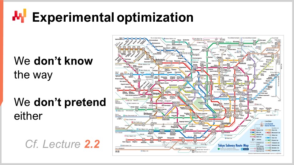
When the word “optimization” is pronounced, the usual perspective that comes to mind for a well-educated audience is the mathematical optimization perspective. Given a set of variables and a loss function, the goal is to identify variable values that minimize the loss function. Unfortunately, this approach works poorly in supply chain because it assumes that the relevant variables are known, which is usually not the case. Even when it is the case, there are plenty of variables, like weather data, that are known to have an impact on your supply chain but come with a lot of costs if you want to acquire this data. Thus, it’s not clear if it’s worth the effort to acquire this data to optimize your supply chain.
Even more troublesome, the loss function itself is largely unknown. The loss function can be guesstimated somehow, but only the confrontation of the loss with the real-world feedback that you can obtain from your supply chain will give you valid information about the adequacy of this loss function. It’s not a matter of correctness from a mathematical perspective; it’s a matter of adequacy. Does this loss function, which is a mathematical construct, adequately reflect what you’re trying to optimize for your supply chain? We addressed this conundrum of performing optimization while we don’t know the variables and the loss function in Lecture 2.2, titled “Experimental Optimization.” The experimental optimization perspective states that the problem is not a given; the problem must be discovered through repeated, iterated experiments. The proof of the correctness of the loss function and its variables emerges not as a mathematical property but through a series of observations driven by well-chosen experiments obtained from the supply chain itself. Experimental optimization profoundly challenges the way we look at optimization, and this is a perspective that I will be adopting in this chapter. The tools and techniques that I will be introducing here are geared toward the experimental optimization perspective.
At any point in time, the numerical recipe that we have can be declared obsolete, and it can be replaced by an alternative numerical recipe that is deemed to be more closely aligned with the supply chain we have. Thus, at any point in time, we should be able to put the numerical recipe we have into production and perform the optimization process at scale. For example, we cannot say we identify the loss function and then put a team of data scientists on the case for three months to engineer some software optimization techniques. Instead, whenever we have a new recipe, we should be able to directly put it into production and immediately let the supply chain decisions benefit from this newly identified form of the problem.

This lecture is part of a series of supply chain lectures. I’m trying to keep these lectures somewhat independent, but we are past a point where it makes more sense to watch these lectures in sequence. If you have not watched the previous lectures, it should be okay, but this series will probably make more sense if you watch it in the order it was presented.
In the first chapter, I presented my views on supply chain both as a field of study and as a practice. In the second chapter, I presented a series of methodologies essential for tackling supply chain challenges, including experimental optimization. These methodologies are needed because of the adversarial nature of most supply chain problems. In the third chapter, I focused on the problems themselves, as opposed to the solutions. In the fourth chapter, I presented a series of fields that are not exactly supply chain per se – the auxiliary sciences of supply chain – which are essential to a modern practice of supply chain. In the fifth chapter, I presented a series of predictive modeling techniques, most notably probabilistic forecasts, which are essential to cope with the irreducible uncertainty of the future.
Today, in this first lecture of the sixth chapter, we delve into decision-making techniques. The scientific literature has delivered an abundance of decision-making techniques and algorithms over the last seven decades, from dynamic programming in the 1950s to reinforcement learning and even deep reinforcement learning. The challenge, however, is to achieve production-grade supply chain results. Indeed, most of these techniques suffer from hidden flaws that make them impractical for supply chain purposes for one reason or another. Today, we focus on retail stock allocation as the archetype of a supply chain decision. This lecture paves the way for more complex decisions and situations.
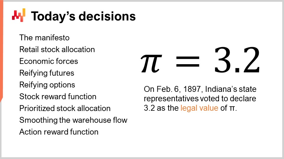
On the screen is the summary for today’s lecture. Even when considering the simplest supply chain problem, retail stock allocation, we have quite a lot of ground to cover. These elements represent building blocks for more complex situations. I will start by revisiting the manifesto of quantitative supply chain. Then, I will clarify what I mean by the retail stock allocation problem. We will also review the economic forces present in this problem. I will revisit the notion of probabilistic forecasts and how we actually represent them, or at least one of the options to represent them. We will see how to model the decision by refining the forecast and refining the options, which are the candidate potential decisions.
We will then introduce the stock reward function. This function can be seen as a minimal framework to convert a probabilistic forecast into an economic score that can be associated with every stock allocation option, taking into account a series of economic factors. Once the options are scored, we can proceed with a priority list. A priority list is deceptively simple but proves to be incredibly powerful and practical in real-world supply chains, both in terms of numerical stability and white-boxing characteristics.
With the priority list, we can almost effortlessly smooth the flow of inventory from the distribution center to the stores, reducing the operating cost of the distribution center. Finally, we will briefly survey the action reward function, which nowadays supersedes the stock reward function at Lokad in virtually every dimension, except simplicity.
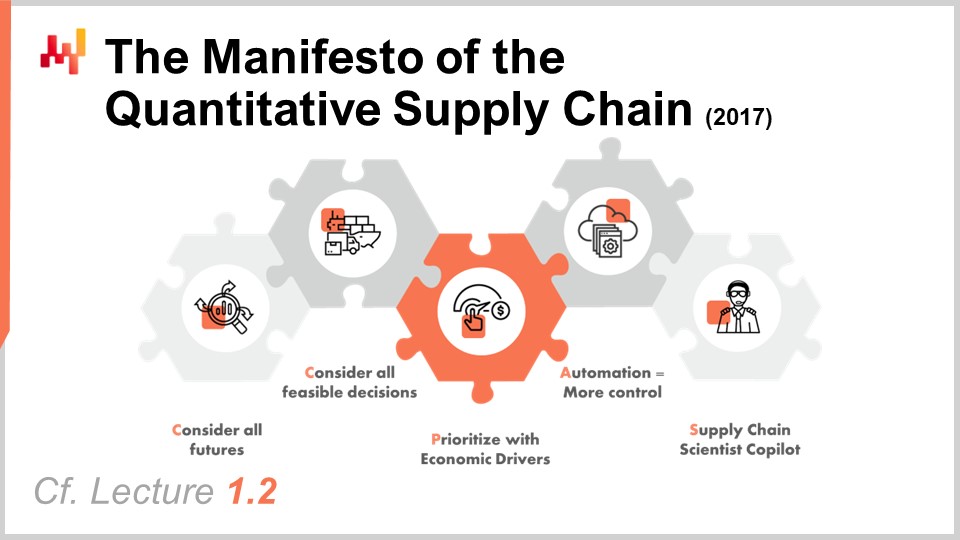
The manifesto of the quantitative supply chain is a document that I originally published in 2017. This perspective has been extensively covered in Lecture 1.2, but for the sake of clarity, I will provide a brief recap today. There are five pillars, but only the first three are relevant for us today. The first three pillars are:
Consider all possible futures, which means probabilistic forecasts as well as forecasting all other elements with an aspect of uncertainty, such as varying lead times or future prices. Consider all feasible decisions, focusing on decisions and not artifacts. Prioritize with economic drivers, which is the topic of today’s lecture.
In particular, we will see how we can convert probabilistic forecasts into estimates of economic returns.
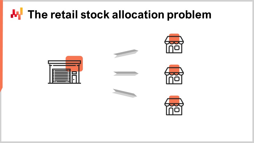
In the retail stock allocation problem. This is a definition that I’m giving; it is somewhat arbitrary, but this is the definition that I will be using today. We assume a network with two echelons: we have a distribution center and multiple stores. The distribution center is serving all the stores, and if there are multiple distribution centers, we assume that one store is served by only a single distribution center. The goal is to properly allocate the stock that exists in the distribution center among the stores, and all the stores compete for the same stock that exists in the distribution center.
We assume that all stores can be replenished on a daily basis with a daily schedule from the distribution center. Thus, every single day, we must decide how many units to move for every single product toward each store. The total quantity of units that are moved cannot exceed the stock available in the distribution center, and it is also reasonable to expect that there are store shelf capacity limits. If the distribution center had unlimited stocks, the problem would devolve into a single-echelon supply chain, as there would never be any need to do any kind of arbitrage or trade-off between allocating the stock to one store or another. The two-echelon property of the network only emerges due to the fact that the stores compete for the same stock.
Naturally, we will assume visibility on the store sales and the stock levels both at the distribution center level and the store level, meaning we assume the transactional data is available. We will also assume that the incoming deliveries to be made at the distribution center are known with estimated times of arrival (ETAs), which may come with some degree of uncertainty. We also assume that all the mundane but critical information is available, such as the product buy price, the product sell price, the product categories if any, etc. All of this information would be found in any ERP, even three decades old, as well as WMS and point-of-sale systems.
Today, we do not include the distribution center (DC) replenishment as part of the problem. In practice, distribution center replenishment and store allocations are tightly coupled, so it makes sense to address those problems together. The reason why I’m not doing that today is for the sake of clarity and concision in this lecture; we will tackle the simpler problem first. However, please note that the approach that I’m presenting today can be naturally extended to include the DC replenishment as well.
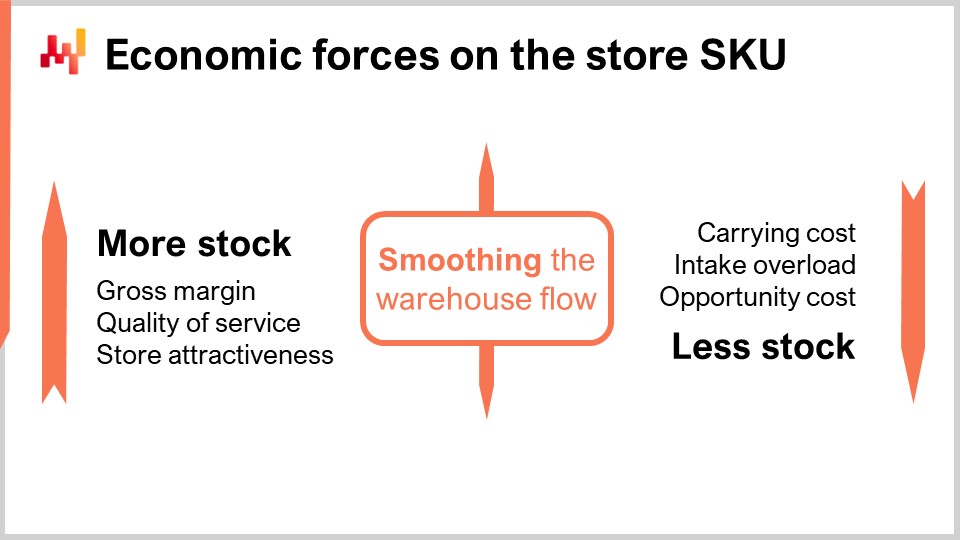
Deciding to move plus one unit of stock into a store for a given product at a given day depends on a series of economic forces. If moving the unit is profitable, we want to do it; otherwise, we don’t. The main economic forces are listed on the screen, and essentially, putting more stock in a store results in a series of benefits. These include more gross margin due to avoiding lost sales, better quality of service by reducing the amount of stockouts, and improved store attractiveness. Indeed, for a store to be attractive, it needs to appear plentiful; otherwise, it looks sad and people may be less willing to buy. This is a common observation in retail, although it may not necessarily apply to all segments, such as hard luxury. For general merchandise or fashion stores, however, this consideration applies.
Unfortunately, putting more stock also comes with drawbacks, diminishing the return that could be expected from having more stock in the store. These drawbacks include extra carrying costs, which can turn into inventory write-offs if there is a true excess of stock. There is also the risk of intake overload, which occurs if the staff at the store cannot process a shipment that is too large. This creates confusion and disorder in the store if the quantity being delivered exceeds what the staff can put on the shelves. Additionally, there is an opportunity cost: whenever a unit is placed in one store, it cannot be put into another store. While it could be brought back to the distribution center and resent, this is typically quite expensive, so it is usually a last resort option. Retailers should aim for efficient store allocation without having to move stock back.
Smoothing the flow of inventory is also highly desirable. A distribution center (DC) has a nominal capacity at which it operates at peak economic efficiency. This peak efficiency is driven by the physical setup of the DC, as well as the number of permanent staff attached to it. Ideally, the DC should operate on a daily basis, remaining very close to its nominal capacity to be most cost-efficient. However, maintaining peak efficiency at the distribution center (DC) requires smoothing the flow from the DC to the stores. The economic perspective diverges from the traditional service level-oriented perspectives often seen in mainstream supply chain literature. We are seeking dollars of return, not percentage points. The only way to decide if it’s reasonable to adjust the stock allocation scheme at the network level to reduce operating costs, versus a minor degradation of quality of service in stores, is to adopt the economic perspective presented here. If you adopt a service-level perspective, it cannot provide these sorts of answers. Our goal at this point is to establish numerical recipes that will estimate the economic outcomes for any given stock allocation decision.
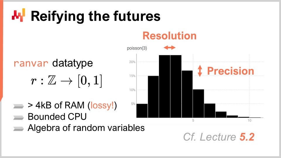
In the previous chapter, the fifth chapter, we discussed how to produce probabilistic forecasts and introduced a specialized data type, the “ranvar,” which represents one-dimensional discrete probability distributions. In short, a ranvar is a specialized data type used to represent a simple one-dimensional probabilistic forecast in Envision.
Envision is a domain-specific programming language engineered by Lokad for the sole purpose of predictive optimization of supply chains. While there is nothing fundamentally unique about Envision in these lectures, it is used for presentation clarity and concision. The numerical recipes described today can be implemented in any language, such as Python, Julia, or Visual Basic.
The key aspect of ranvar is that it provides a high-performance algebra of random variables. Performance is a balance between compute cost, memory cost, and the degree of numerical approximation you are willing to tolerate. Compute performance is critical when dealing with retail networks, as there can be millions or even tens of millions of SKUs, each likely to have at least one probabilistic forecast or ranvar. Consequently, you may end up with millions or tens of millions of histograms.
The key property of ranvar versus a histogram is to keep both CPU cost and memory cost upper bounded and as low as possible. It is also crucial to ensure that the numerical approximation introduced remains inconsequential from a supply chain perspective. It is important to note that we are not dealing with scientific computing here, but supply chain computation. While numerical calculations should be precise, there is no need for extreme precision. Keep in mind that we are not doing scientific computing here; we are doing supply chain computation. If you have an approximation of one part per billion, it is inconsequential from a supply chain perspective. Numerical calculations should be precise, but there is no need for extreme precision.
In the following, we assume that the probabilistic forecast will be provided under the guise of ranvars, which are a series of variables with a specific data type. In practice, you can replace ranvars with histograms and achieve mostly the same outcome, except for the performance and convenience aspects.
Now that we have our probabilistic forecasts, let’s consider how we will approach the decisions. Let’s start by considering the options. The options are the potential decisions – for example, allocating zero units for a given product to a given store on a given day or allocating one, two, or three units. If we decide to allocate two units, then that becomes our decision. The options are all the things on the table waiting to be decided.
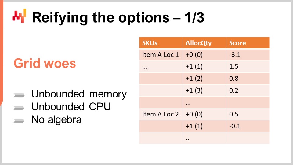
A simple way to organize these options is to put them in a list, as displayed on the screen. The list covers multiple SKUs, and for every SKU, you add one line per option. Each option represents a quantity to be allocated. You can allocate zero, one, two, three, and so on. In reality, you don’t have to go to infinity; you can stop at the quantity in stock at the distribution center. More realistically, you usually have a lower bound, such as the maximal shelf capacity for the product in the store.
So, you have a list that includes every SKU, and for every SKU, you have all the quantities that can be considered as candidates for allocation from the distribution center. The score column is attached to the marginal outcome you would expect by making this allocation. A well-designed score ensures that picking lines in decreasing score order optimizes the economic outcome for the retail network.
For the two SKUs shown on the screen, the score decreases as the allocation increases, illustrating the dominant phenomenon of diminishing returns observed for most SKUs. Essentially, putting the first unit in a store almost always generates more returns than the second one. The first unit that you put in a store is almost always more profitable than the second one. Initially, you have nothing, so you’re in a stock-out situation. If you put one unit, you’ve already addressed the stock-out for the first client. If you put a second unit, the first client will be fine, but it’s only if two clients show up that the second unit will be of any use, so it has a smaller economic return. However, the returns are generally diminishing as you increase the stock. There are some exceptions where the economic returns might not be strictly diminishing from one line to the next, but I will revisit this case in a later lecture. For now, we’ll stick to the simple situation where the returns are strictly diminishing as stock increases.
The representation we have, where we can see all the SKUs and options, is typically referred to as a grid. The intent is to sort this grid by decreasing ROI (return on investment). There is nothing wrong with these grids per se, but they are not very efficient, especially compute-wise or memory-wise, and they don’t offer any support beyond being a large table. Keep in mind that we are talking about a retail network, and this grid might end up having a billion lines or so. Big data is fine, but smaller data is better, as it creates less friction and allows for more agility. We want to try to turn our big data problem into a small data problem, as smaller data makes everything simpler in production.
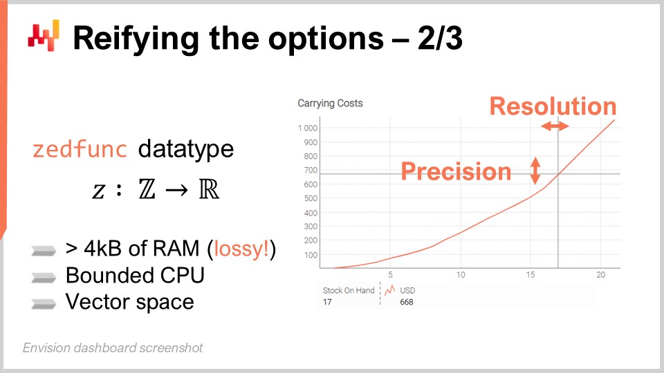
Thus, one of the solutions adopted by Lokad to deal with a large number of options is zedfuncs. This data type, just like ranvars, is the counterpart of ranvar but from the decision perspective. ranvars represent all the possible futures, while zedfuncs represent all the possible decisions. Instead of representing probabilities like ranvars, a zedfunc represents all the economic outcomes associated with a one-dimensional discrete series of options.
The zedfunc, or zedfunction, is technically a function mapping integers, both positive and negative, to real values. This is the technical definition. However, just like with ranvars, it is not possible to represent any arbitrary or complex function like zedfuncs with a finite amount of memory. In this case, there is also a trade-off to be made between precision and resolution.
In supply chain management, arbitrarily complex economic functions do not exist. You can have fairly complex cost functions, but they cannot be arbitrarily complex. In practice, it is possible to compress zedfuncs under four kilobytes. By doing so, you have a data type that represents your entire cost function and compresses it so that it always stays less than four kilobytes while keeping the degree of numerical approximation inconsequential from a supply chain perspective. If you keep the numerical approximation so small that it doesn’t change the final decision you’re about to make, which is discrete, then the numerical approximation can be said to be completely inconsequential because you end up doing the same thing in the end, even if you had infinite precision.
The reason for using four kilobytes is related to computing hardware. As we have seen in a previous lecture about modern computing hardware for supply chain management, the random access memory (RAM) in a modern computer, be it a workstation, notebook, or a computer in the cloud, doesn’t let you access memory byte per byte. As soon as you touch the RAM, a segment of four kilobytes is retrieved. Therefore, it is best to keep the amount of data under four kilobytes because it will match the way the hardware is designed and operates for your supply chain.
The compression algorithm used by Lokad for zedfuncs differs from the one used for ranvars because we are not addressing the same numerical problems. For ranvars, we mostly care about preserving the mass of probabilities of our contiguous segments. For a zedfunc, the focus is different. We typically want to preserve the amount of variation observed from one position to the next because it is with this variation that we can decide whether it is the last profitable option or if we should stop. Therefore, the compression algorithm is different as well.
On the screen, you can see a plot obtained for a zedfunc reflecting some expected carrying costs that depend on the number of units in stock. zedfuncs benefit from being a vector space, meaning they can be added and subtracted, just like the classical vector space associated with functions. By preserving memory locality, operations can be performed an order of magnitude faster compared to a naive grid implementation where you have a very large table without a specific data structure to capture the locality of the options playing together.
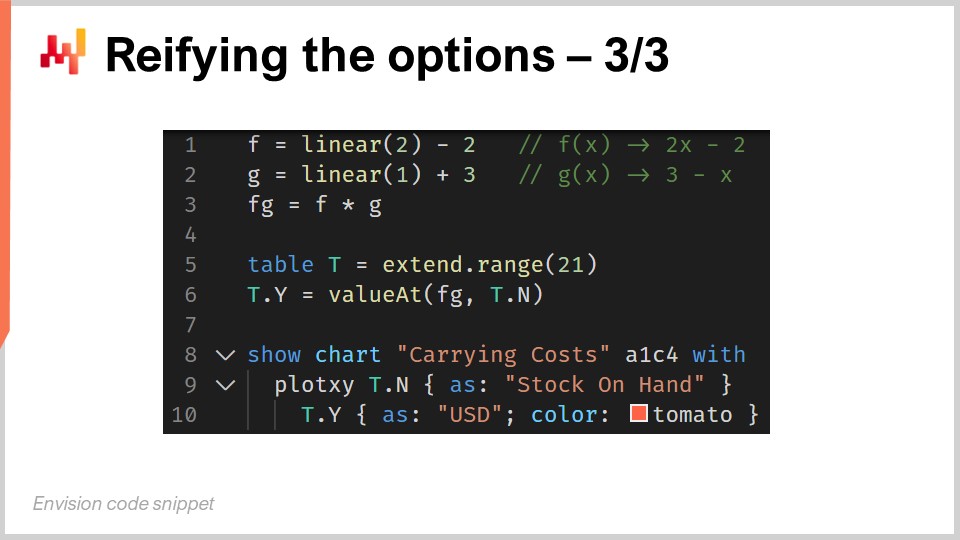
The plot you saw in the previous slide was generated by a script. At lines one and two, we declare two linear functions, f and g. The function “linear” is part of the standard library, and “linear of one” is just the identity function, a polynomial of degree one. The function “linear” returns a zedfunc, and it is possible to add a constant with a zedfunc. We have two polynomials of degree one, f and g. At line three, we construct a second-degree polynomial through the product of f and g. Lines 5 to 10 are utilities, essentially boilerplate, to plot the zedfunc.
At this point, we have our data container for the zedfunc and the economic outcomes. The zedfunc is a data container, just like the ranvar was for the probabilistic forecast. However, we still need numerical recipes to compute those economic outcomes. We have the data container, but I haven’t described yet how we compute those economic outcomes and fill in the zedfuncs.
The stock reward function is a small framework intended to compute the economic returns for every stock level of a single SKU, considering a probabilistic forecast and a short series of economic factors. The stock reward function was historically introduced at Lokad to unify our practices. Back in 2015, Lokad had already been working for a couple of years with probabilistic forecasts, and through trial and error, we had already uncovered a series of numerical recipes that worked well. However, they were not really unified; it was a bit of a mess. The stock reward function consolidated all those insights at the time into a clean, tidy, minimalistic framework. Since 2015, better methods have been developed, but they are also more complex. For the sake of clarity, it’s still better to start with the stock reward function and present this function first.
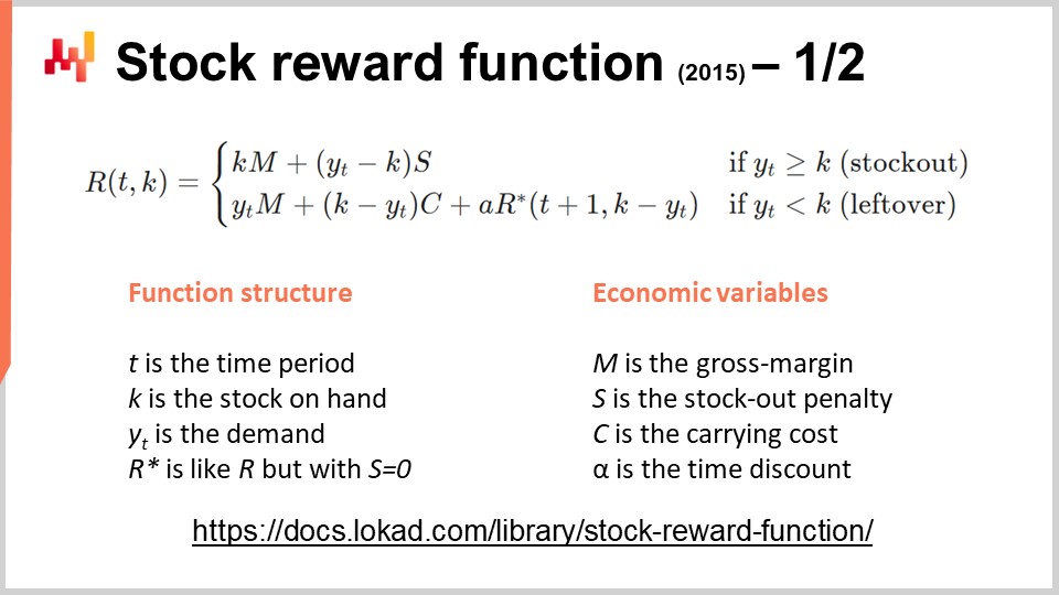
The stock reward function is really about finding a numerical recipe that will give us a calculation for the economic outcomes attached to those probabilistic forecasts. The stock reward function obeys the equation you can see on the screen, and it defines the economic returns at time t that you can obtain for the stock on hand, k. The variable R represents the economic return, which is expressed in units such as dollars or euros. The function has two variables: time (t) and stock on hand (k). We want to compute this reward for all possible stock levels.
There are four economic variables to be considered:
M is the gross margin per unit sold. It’s the margin you will earn by successfully servicing one unit. S is the stockout penalty, a sort of virtual cost that you incur whenever you fail at servicing a unit to a client. Even if you don’t have to pay a penalty to your client, there is a cost associated with failing to provide proper service, and this cost must be modeled. One of the simplest ways to model this cost is to assign a penalty for every unit that you fail to serve. C is the carrying cost, the cost per unit per period of time. If you have one unit in stock for three periods, that would be three times C; if you have two units in stock for three periods, that would be six times C. Alpha is used to discount future returns. The idea is that what happens in the distant future matters less than what is about to happen in the near future. The stock reward function is as simple as it can be without being overly simplistic. The equation indicates that if demand exceeds the stock on hand, the return includes the margin for all the stock we have.
This is what the first line is saying: we have k margins, so we sell all the units we have, and then we incur a penalty that’s going to be Y(t) - k for all the units we failed to serve.
Otherwise, if the stock on hand exceeds the demand, we can benefit from Y(t) times M, which represents the margin of what we have sold today. Then, we have to pay for the carrying costs. The carrying costs for today will be what is left at the end of the day, which is k - Y(t) times C, plus alpha times the stock reward function R* for the next day.
There is a catch with R*. It is almost identical to the stock reward function R, except that we just put the stockout penalty at zero. The reason is straightforward: we assume from the stock perspective that we will have later opportunities to fill in the stock. If we observe a stockout today, it is too late, so we do incur the stockout penalty. However, a stockout penalty that is deemed to occur tomorrow is considered avoidable.
However, a stockout penalty that is deemed to occur in the future, in a later period, we assume that replenishment can happen at every period. Thus, for the stockout that would happen at a later period, when we still have time to do a late reorder, the stockout has not yet happened. We still have the opportunity to do it, and that’s why we put the stockout penalty at zero, because we anticipate that there will be, hopefully, another reorder that will prevent the stockout from happening.
The time discount alpha is very useful because it essentially removes the need to specify a specific time horizon. The stock reward function doesn’t work with a finite time horizon; you go till infinity. Thanks to alpha, which is a value that is strictly smaller than one, the economic outcomes attached to events in the very distant future become vanishingly small, so they become inconsequential. We don’t have any kind of cutoff, which is always arbitrary, such as cutting your supply chain horizon to 60 days, 90 days, one year, or two years.
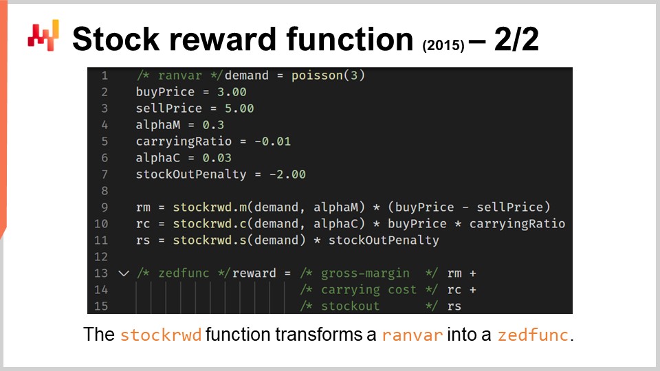
In Envision, the stock reward function takes a ranvar as input and returns a zedfunc. The stock reward function is a small building block that turns a probabilistic forecast (a ranvar) into a zedfunc, which is a container for the estimated economic returns on a series of options. As the name suggests, the stock reward function is the economic return associated with every single stock position: what happens if I have zero units in stock, one unit in stock, two units, three units, and so on. The zedfunc will reflect the economic outcomes for each stock level, encoding the economic return associated with the corresponding stock level.
The process to compute these zedfuncs is illustrated on the screen. At line 1, we introduce a mock demand for a single day, which is just a random Poisson distribution. At lines 2 to 7, we introduce the economic variables, and by the way, we have two alphas. There is another catch: we have a ratchet effect on the inventory. Once the stock has been pushed toward the store, it is typically very expensive to bring the stock back. This reflects that any allocation made to a store is pretty much final. In terms of carrying costs, the alpha should not be too small, because we will really incur those carrying costs if we overstock. We cannot undo this decision. However, when it comes to the alpha that is related to the margin, the reality is that just like we will have other opportunities to address future stockouts, we will have other opportunities to bring more stock and perform the same margin with stock that is pushed at a later date. Thus, we need to discount much more aggressively whatever happens on the margin side compared to what is happening on the carrying cost side.
At lines 9 to 11, we introduce the stock reward function itself. This function, the stock reward function that I introduced in the previous slide, can be decomposed linearly into its three components, respectively addressing the margin, the carrying cost, and the stockout penalty separately. Indeed, we have a linear separation, and in Envision, these three components are computed separately. We can multiply the zedfunc by the factor M, which would be the gross margin.
At lines 13 to 15, the final reward is recomposed by adding the three economic components. In this script, we are leveraging the fact that we have a vector space of zedfuncs. These zedfuncs are not numbers; they are functions. But we can add them, and the result of the addition is another function, which is also a zedfunc. The variable reward is the result of adding those three components together. Under the hood, the calculation of the stock reward function is done through a fixed-point analysis, which can be done in constant time for every component. This constant time calculation might seem like a minor technicality, but when you’re dealing with a large retail network, it makes the difference between a fancy prototype and an actual production-grade solution.
Now, at this point, we have consolidated all the ingredients needed to address the stock allocation problem. We have probabilistic forecasts expressed as ranvars, a technique to transform these ranvars into a function giving economic returns for any stock on hand value, and those economic outcomes can be conveniently represented as zedfuncs. To finally address the stock allocation problem, we need to answer the key question: if we can only move one single unit of stock, which one do we move and why? All the stores in the network are competing for the same stock in the distribution center, and the quality of the decision of moving one unit of stock from the distribution center to a specific store depends on the overall state of the network. You cannot assess whether this decision is good by just looking at one store.
For example, let’s assume we have a store with already two units in stock, and if we add a third unit, we are increasing the expected service level from 80% to 90%. This is good, and maybe more within the network would agree with the idea of bringing one extra unit so that the service level can go from 80 to 90. That seems very reasonable, so they would say this is a good move. However, what if this unit we are about to move, this third unit, is actually the last one available in the distribution center? We have another store on the network that is already suffering a stockout, and if we move this unit into the store where it becomes the third unit, we prolong the stockout for the store that is already out of stock for the same product. In this situation, it is almost certain that moving the unit to the store already out of stock is a better decision and should take a higher priority.
That’s why it doesn’t make sense to assess economically stock levels at the SKU level. The problem with local optimizations is that they don’t work if you operate in larger systems. In supply chains, if you address things locally, you just displace problems; you don’t address anything. The adequacy of a stock level of an SKU is dependent on the state of the network. This simple example clarifies why safety stock calculations or reorder point calculations are mostly nonsense, at least for real-world situations, compared to toy examples found in supply chain textbooks.
Here, we really want to prioritize all the stock allocations against one another, and the option that comes out on top is the answer to our question: this will be the one unit that should be moved if we can only move a single unit.
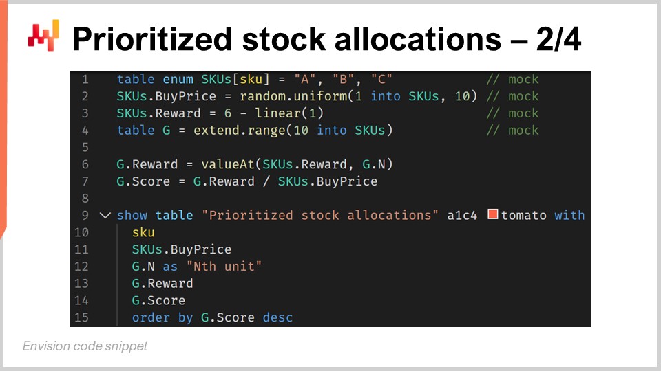
Ranking stock allocation options is relatively straightforward with the proper tools. Let’s review this Envision script. At line 1, we create three SKUs named A, B, and C. At line 2, we generate random buy prices between 1 and 10 as mock data. At line 3, we generate mock zedfuncs that are supposed to represent the reward we have for each of those SKUs. In practice, a zedfunc should be computed with the stock reward function, but just to keep the code concise, we are using mock data here. The reward is a decreasing linear function that will hit zero at stock level 6. At line 4, we create a table G, a shorthand for the grid that represents our stock on hand levels. We assume that stock levels above 10 are not worth assessing. This assumption is reasonable, considering that in terms of mock data, we have a reward function that becomes negative beyond a stock-on-hand level of 6. At line 6, we extract the marginal reward for any unit in stock so that we have this grid table. We use the zedfunc, a function that represents rewards, to extract the value for the stock position G.N. It’s worth noting that starting from line 6, it wouldn’t matter how the data was originally generated. From line 1 to 4, it is just mock data that wouldn’t be used in a production setup, but starting from line 6, it would be essentially the same if you were in production.
At line 7, we define the score as a ratio between the dollars of returns (which the zedfunc tells you) and the dollar invested, which is the buy price. We make a ratio between the amount of dollars that you will get back divided by the amount of dollars you have to pay for one unit. Essentially, the highest score is obtained for the stock allocation that generates the highest rate of return per dollar allocated to this store.
Finally, at lines 9 to 15, we display a table sorted by decreasing scores. It’s important to point out that there is no fancy logic in the script. The first four lines are just mock data generation, and the last six lines are just the display of prioritized allocation. Once the zedfuncs are present and we have a function that represents economic returns per stock level, turning those zedfuncs into a prioritized list is completely straightforward.
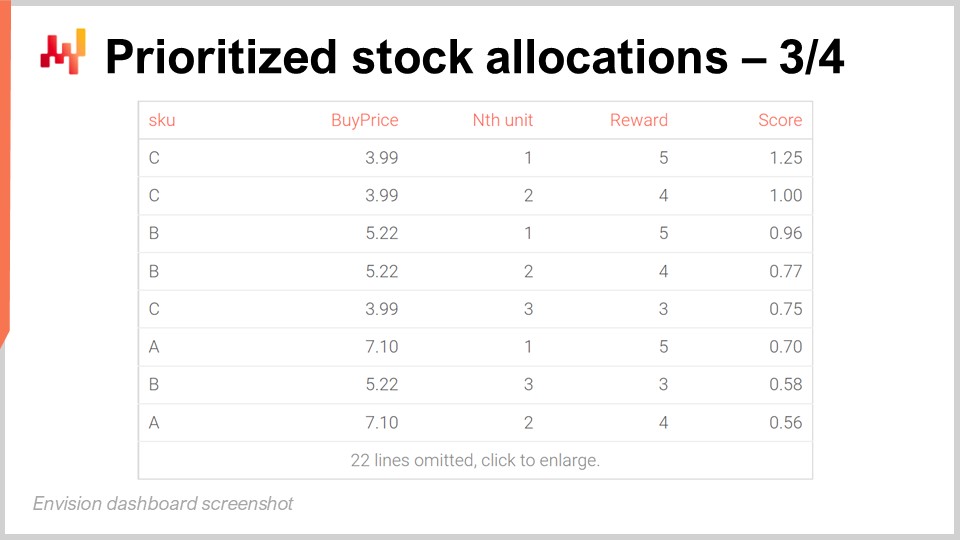
On the screen, the table obtained by running the previous Envision script shows that the SKU named C is ranked first. All the SKUs have the same economic returns for their first unit, namely $5 of return. However, C has the lowest buy price at $3.99, and thus, when we divide the reward of $5 by $3.99, we get a score of approximately 1.25, which happens to be the highest score on the grid. The second unit of C has a score of approximately 1, which is the second-highest score.
For the third position in the grid, we have another SKU named B. B has a higher buy price, and thus its score for the first unit is only at 0.96. However, due to the diminishing returns that we get from allocating the first two units to SKU C, the first unit of B gets a higher score than the third unit of C, and thus it gets ranked above the third unit of C. Essentially, this priority list goes very deep, but it is intended to be truncated with a threshold. For example, we can decide that there is a minimal return on investment, and only the units above this return on investment get allocated. Once the threshold is defined, we can take all the lines that are above the cutoff and count the number of lines per SKU. This gives us the total number of units to be allocated for every single SKU. We will revisit this cutoff problem in a minute, but the idea is that once you have a cutoff, you aggregate the counts per SKU, and that gives you the total quantity to be allocated for every single SKU. This is exactly what your WMS or ERP that exists in the distribution center would expect to organize the next day’s shipment toward the stores.
The priority list is just a conceptual view to actually decide what takes priority. However, you take a cutoff, aggregate, and then you’re back to allocation quantities per SKU for every single SKU that exists in your retail store network.
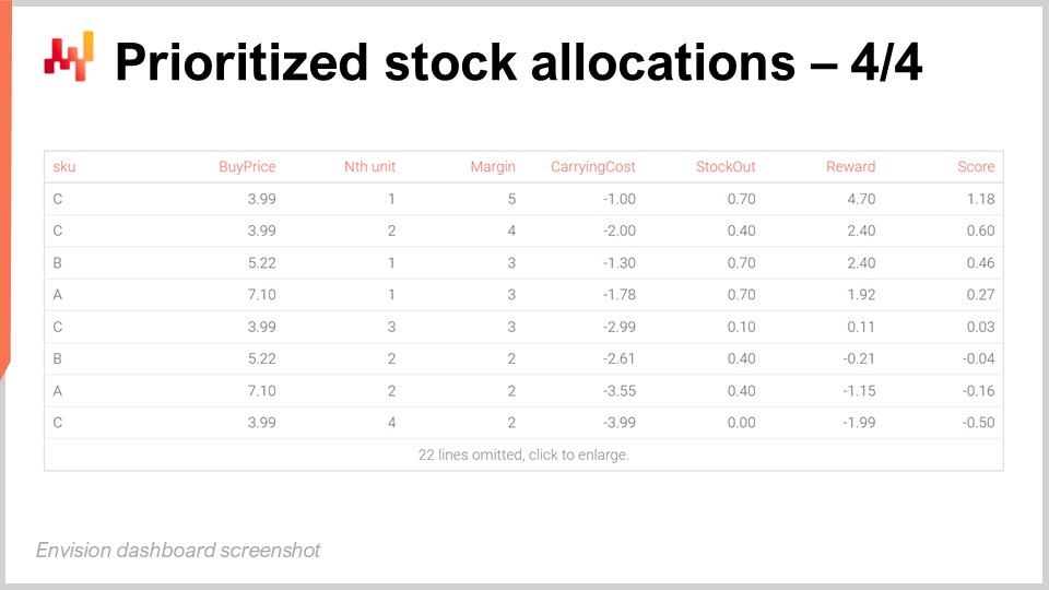
The view on the display of prioritized stock allocation is deceptively simple and yet powerful. As we go down from one line to the next, we see the competition unfold between our allocation options. The best SKUs get allocated first, but as soon as we reach higher stock levels, those SKUs become less competitive compared to other SKUs that don’t have as much stock. The priority list switches from one SKU to the next, maximizing the expected returns on capital being allocated to the stores.
On this screen, we have a variant of the previous table, obtained with another Envision script that is a minimal variant of the one introduced two slides ago. Essentially, I am decomposing the economic factors that contribute to the reward. Here we have three extra columns: margin, carrying cost, and stockout. The margin is the expected average gross margin for this one unit being allocated. The carrying cost is the expected average cost of putting this one unit in the stock in the store. The stockout is the expected penalty that is going to be avoided, which is why the stockout penalty is a positive value here. The final reward is just the sum of those three components, and all those values are expressed in monetary amounts, such as dollars. The column that is margin dollars, carrying cost dollars, and stockout dollars, and rewards, is just the total amount of dollars that you can expect by putting this one unit into the store.
This makes understanding and debugging this numerical recipe, expressed in dollars, vastly easier compared to percentages.Indeed, any non-trivial numerical recipe is going to be fairly opaque by design. You don’t need deep learning to get deep opacity; even a modest linear regression is going to be plenty opaque as soon as you have a couple of factors that are involved in this regression. This opacity, which you get again with any non-trivial numerical recipe, puts a real-world supply chain at risk because supply chain practitioners can get lost, confused, and distracted by modeling technicalities.
The prioritized list of allocation, which decomposes the economic drivers, is a powerful audit tool. It lets the supply chain practitioners directly challenge the fundamentals instead of muddling through the technicalities. You can directly ask questions like: Do we have carrying costs that make sense considering the situation we are in? Are those costs aligned with the sort of risks we are taking? You can forget the forecast, the seasonality, and the way you model the seasonality, the way you factor the decreasing trend, and whatnot. You can directly challenge the final outcome, which is dollars of outputs for those carrying costs. Are they real? Do they make sense? Very frequently, you can spot numbers that are nonsensical and fix them directly.
Obviously, you want to avoid those situations, but don’t operate under the assumption that in supply chain all the problems are incredibly subtle forecasting problems. Most of the time, the problems are brutal. There may be some kind of issue, such as data not being processed correctly, and then you get numbers that are completely nonsensical, such as negative margins or negative carrying costs that wreak havoc in your supply chain.
If your supply chain instrumentation exclusively focuses on demand forecasting accuracy, you are blind to 90% (or more) of the actual problems. In a large-scale supply chain, this estimate would probably be something like 99%. Supply chain instrumentation is absolutely fundamental to highlight the key factors that contribute to the decisions, and those factors must be economic in nature if you want to have any hope of focusing on what makes your company profitable. Otherwise, if you operate on percentages, you can’t prioritize your own actions, and you will address glitches indiscriminately. We are talking about a large-scale supply chain, so there is always a legion of numerical glitches. If you address all those glitches indifferently, it means that you’re always working on things that are largely inconsequential. That’s why you need to have dollars of returns and dollars of cost. That’s how you can actually prioritize your work and your development efforts for your numerical recipes. Sometimes, you don’t even need to decide whether a bug is worth fixing; if you’re talking about a handful of dollars per year worth of friction, it’s not even a bug that is worth fixing in practice.
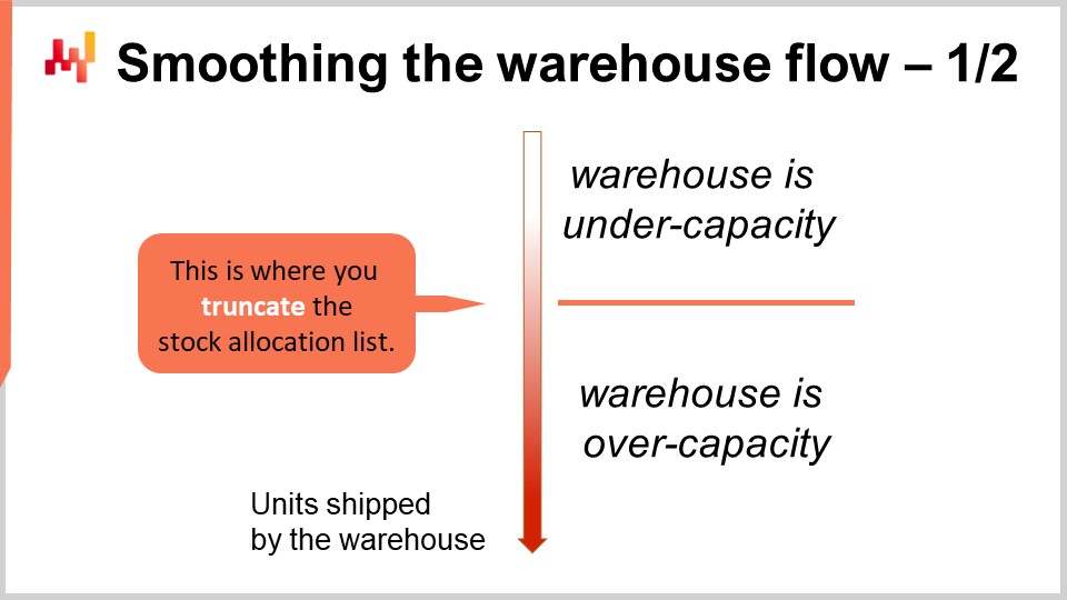
Now, let’s get back to the matter of picking the right cutoff for the allocation list. We have seen that we have roughly diminishing returns while allocating more stock to the store SKUs. However, we must look at the whole supply chain, not just the warehouse or distribution center. I’m using the two terms interchangeably here. The warehouse or distribution center is dominated by fixed costs. Indeed, it is possible to extend the staff with temp workers, but it tends to cost more, and it creates other problems, such as the temp workforce being typically less qualified than the permanent one.
Thus, any warehouse or any distribution center has a target capacity where it operates at peak economic efficiency. The target capacity can be increased or decreased, but usually, it involves adjusting the size of the permanent staff, so it is a relatively slow process. You can expect a warehouse to adjust its target capacity from one quarter to the next, but you can’t expect the warehouse to adjust its nominal capacity, where it has peak efficiency, from one day to the next. It’s not as dynamic.
We want to keep the warehouse operating at peak efficiency, or as close as possible to peak efficiency, all the time, unless we have an economic incentive that is strong enough to do otherwise. The perspective of the prioritized stock allocation paves the way to do exactly that. We can truncate the list by making it a little shorter or longer and nudging the cutoff to keep it aligned with the target capacity of the warehouse. In practice, this comes with three major benefits.
First, smoothing the flow of the warehouse. By doing this, you keep the warehouse operating at peak capacity most of the time, thus saving a lot of operating costs. Second, your inventory allocation process becomes a lot more resilient to all the little accidents that keep happening in a real-world supply chain. A truck may get involved in a minor traffic accident, some staff may not show up because they are sick – there are tons of small reasons that will disrupt your plans. It will not prevent your warehouse from operating, but it might not operate exactly at the capacity you did anticipate. With this prioritization list, you can make the most of whatever capacity your warehouse happens to be using, even if it’s not exactly the capacity you were planning for in the first place.
The third benefit is that with this approach of a priority list for stock allocation, your supply chain team doesn’t have to micromanage the warehouse staff levels anymore. You only need to adjust the target capacity of your warehouse so that it roughly matches the sales velocity of your retail network. Micromanaging the capacity at a daily level becomes largely inconsequential.
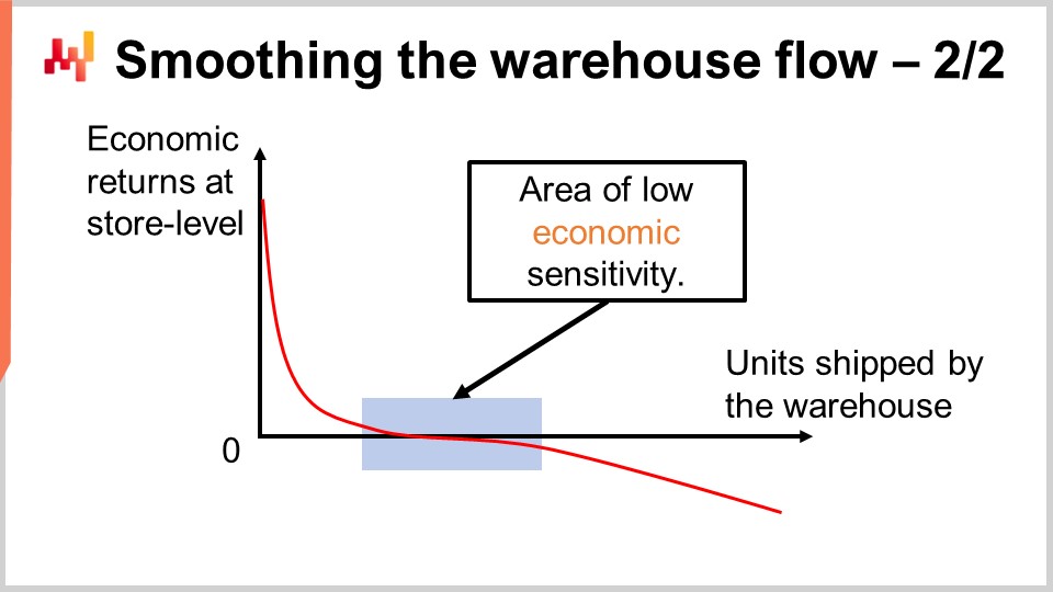
Lokad’s experience indicates that smoothing the warehouse flow through a flat capacity cutoff works well in most retail situations. On the screen, you can see the typical economic return curve that you would observe when considering all the possible cutoffs. On the X-axis, we have the number of units being shipped from the warehouse. We are conceptually assuming that units are shipped one by one so that we can observe the marginal contribution of every single unit. Naturally, in production, units are shipped in batches, not one by one, but this is just so that we can actually plot the curve. On the Y-axis, we have the marginal economic outcomes at the store level, so for the n-th unit being shipped to a store, any store in the network. The very first units being allocated generate the bulk of the returns. In practice, the top of the list invariably consists of stockout situations that demand immediate resolution. That’s why the first units address stockouts, and that’s why the economic returns are very high. Afterward, the returns dwindle, and we enter a flat portion of the curve.
This area is what I refer to as the area of low economic sensitivity. Essentially, we are gradually pushing the service level closer to 100% but are not yet creating much dead stock. When you do this sort of prioritized allocation, if we push stock beyond addressing stockout problems, we end up piling up stock on the fast movers. We create stock in places that are not exactly needed right now. We will have opportunities in the future to replenish the stock without facing a problem of stockout in the meantime, but the impact is minimal because the stock will get sold relatively swiftly. Essentially, this is just about the opportunity cost of moving the stock from the distribution center to a store. We gradually lose future options as we allocate more stock.
This area is relatively flat and will start to become fairly negative when we push so much stock that we start generating situations that will cause inventory write-offs with a non-trivial probability. If you keep pushing, you generate more dire overstock situations, and thus, you see the curve becomes very negative. If you push way too much, you will generate tons of inventory write-offs in the future. As long as the cutoff is in this low sensitivity segment, we’re good, and the cutoff is not super sensitive to where you cut. That’s the reason the warehouse capacity doesn’t have to directly mimic the daily sales volume.
Indeed, in most retail networks, you have a very strong day-of-the-week cyclical pattern that you observe in your sales, where certain days, for example, Saturday, is the day where you’re selling the most. But the warehouse doesn’t have to exactly mimic this day-of-the-week cyclical pattern. You can keep a very flat average, and the idea is that your target capacity should just roughly match your overall sales volume for your store network. If your target capacity is always a little bit below your overall sales volume in the network, what will happen is that you will first deplete all your stores gradually and then face a big problem. Conversely, if you’re pushing every single day a little more than what you’re actually selling, then very quickly, you will completely saturate your stores.
As long as you keep it relatively balanced, you don’t need to micromanage with the day-of-the-week pattern; it will work fine. The reason why you don’t need to micromanage the day-of-the-week pattern is that the very first units deliver the bulk of the returns, and the system from an economic perspective is not that sensitive as long as the cutoff remains roughly in this flattish segment.
Now, I presented the stock reward function for the sake of clarity and concision, as we had much to cover in this lecture already. However, the stock reward function isn’t the pinnacle of supply chain science. It is a bit naive when it comes to the fine print of probabilistic forecasts.
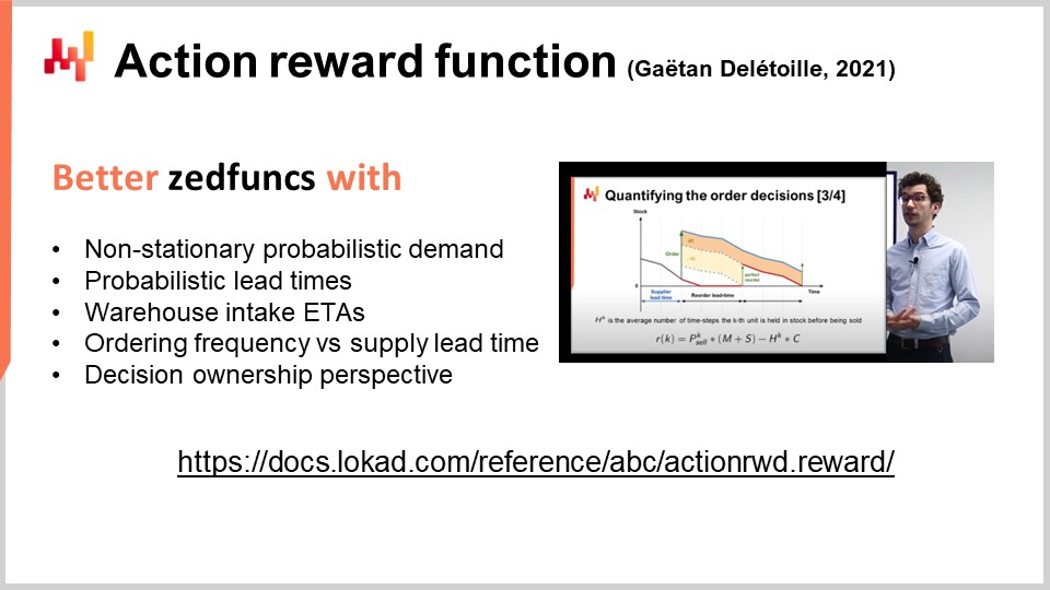
Back in 2021, one of us at Lokad published the action reward function. The action reward function is the spiritual descendant, if you wish, of the stock reward function, but this function comes with a much more fine-grained perspective on the probabilistic forecasts themselves. Indeed, all probabilistic forecasts are not equal. Seasonality, varying lead times, and intake ETAs for the distribution centers are all taken into account in the action reward function, while they were not taken into account with the stock reward function.
By the way, these capabilities also require a more granularistic forecast, so you need superior forecasting technology that can generate all those probabilistic forecasts to make use of the stock reward function. In this regard, the stock reward function is less demanding. At the conceptual level, the action reward function also provides a clean decoupling of the ordering frequency (how frequently you order) from the supply lead time (how much time it takes to replenish the stock once the decision is taken). These two elements were lumped together in the stock reward function. With the action reward, they are clearly separated.
Finally, the action reward function also comes with a decision ownership perspective, which is a simple but fairly clever trick to reap most of the benefits that would be gained from a true policy without having to introduce a policy. We’ll be discussing what policies really mean from a technical perspective in later lectures, but the bottom line is that as soon as you start introducing policies, it becomes more complicated. It is of interest, but it’s definitely more complicated. Here, the action reward has a clever trick where you can literally bypass the need to go for a policy and still reap most of the economic benefits that would be attached to it.
Both the stock reward function and its superior alternative, the action reward function, have been used in production for years at Lokad. These functions essentially streamline entire classes of issues that are otherwise plaguing retail networks. For example, dead stock becomes trivial to assess by just looking at the economic returns attached to any stock unit that is already present in any store. Yet, there are tons of angles that I have not addressed today. I will be addressing those aspects in later lectures.
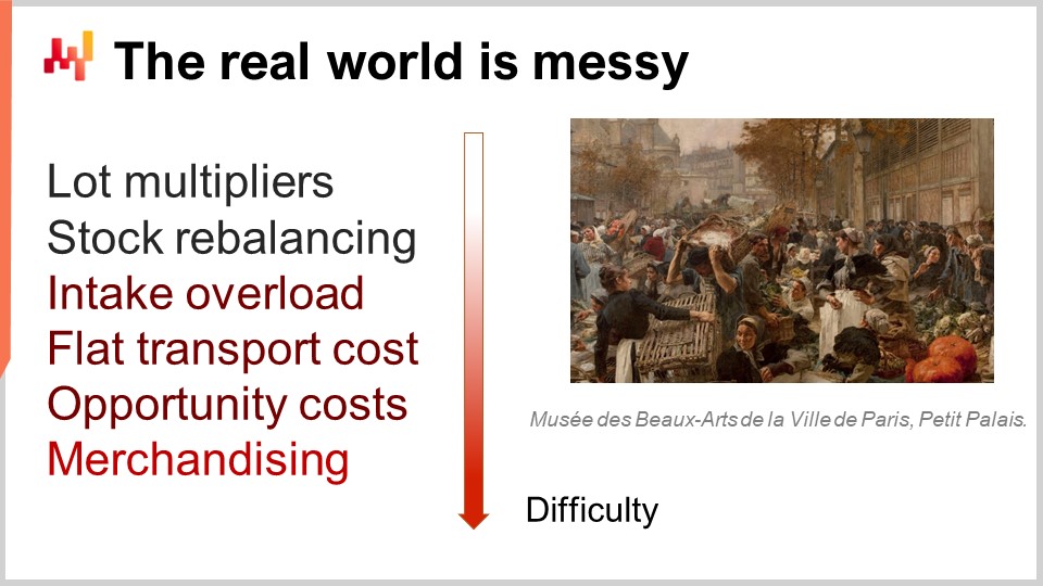
Some of those angles can actually be addressed with fairly minor variations of what I have presented today. That is the case, for example, for lot multipliers and stock rebalancing. You need to do very little change to the scripts I’ve just shown today to be able to tackle those problems. When I say stock rebalancing, I mean rebalance the stock between the stores of the network, either by moving the stock back to the DC or by directly moving the stock between the stores, assuming specific transportation costs.
Then, there are some angles that require more work but are still relatively straightforward. For example, taking into account opportunity costs, flat transportation costs, and store intake overload, which happens when the staff of a store is not capable of processing all the units they have received. They don’t have the time on any given day to put them on the shelves, and thus it creates a big mess in the store. These angles are possible but will definitely require quite some work on top of what I have presented today.
There are other angles, like merchandising or improving the overall store attractiveness, which should be part of the prioritization. These require a superior technological approach, as minor variations of what I’ve presented today are just not enough. As usual, I advise a healthy dose of skepticism whenever an expert claims to have an optimal method. In supply chain, there is no such thing as optimal methods; we have tools, some of them happen to be better, but none of them is even remotely close to anything that would qualify as being optimal.
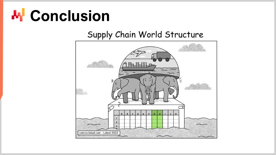
In conclusion, percentages of error are irrelevant; only dollars of error matter. Those dollars are driven by what your supply chain does at a physical level. Most KPIs are inconsequential at best; they are part of the supply chain process to continuously improve the numerical recipes that drive supply chain decisions. However, even when considering such KPIs that are instrumental to improve the numerical recipes, we are talking about fairly indirect results compared to directly improving the numerical recipe that drives the decision and immediately generates better outcomes for your supply chain.
Excel sheets are ubiquitous in supply chain, and I believe this is because the mainstream supply chain theory failed to promote decisions as first-class citizens. As a result, companies waste time, money, and focus on second-class citizens, namely artifacts. But at the end of the day, decisions must be made: stock must be allocated, and you need to choose the price, your selling point, and attack price. Lacking proper support, supply chain practitioners fall back to the one tool that allows them to treat decisions as first-class citizens, and this tool happens to be Excel.
However, supply chain decisions can be treated as first-class citizens, and this is exactly what we did today. The tooling is not even that complex, at least when considering the ambient complexity of the typical applicative landscape of a modern supply chain. Furthermore, adequate tooling unlocks capabilities like smoothing the flow of inventory from distribution centers to the store with minimal effort. These capabilities are straightforward to achieve with the proper tooling but also illustrate the sort of achievements that can never be expected from Excel spreadsheets, at least not with a production-grade setup.
I guess this is it for today. The next lecture will be Wednesday, the 6th of July, at the same time of day, 3 p.m. Paris time. I will be moving on to the seventh chapter to discuss the tactical execution of a quantitative supply initiative. By the way, I will be cycling back to Chapter 5, discussing probabilistic forecasts, and Chapter 6, discussing decision-making techniques, in later lectures. My goal is to have a complete, entry-level perspective on all the elements before going deep into any specific subject.
So at this point, I will actually have a look at the questions.
Question: The zedfunc could have infinite possibilities. Wouldn’t all the solutions be short-term in that case?
The zedfunction is literally a data container for a sequence of options, so the sort of horizon that is applicable is embedded into the alpha value, the time discount values that I’ve used in my scripts. Fundamentally, the target time horizon that you have embedded into the economic outcome of a zedfunction is not really in the zedfunctions themselves; they are more in the sort of economic calculations that are filling them. Don’t forget that the zedfunctions are just data containers. That’s what makes them short-term or long-term, and obviously, you want to adjust your numerical recipes so that they represent your priorities. For example, if your company is under a massive amount of stress due to cash flow problems, you will probably have a much more short-term perspective on having an intake of money, so basically just liquidating your inventory. If you’re very rich in cash, maybe you prefer to delay the sales to a later period, selling at a better price and ensuring a better gross margin. So again, all of those things are possible with zedfunctions. zedfunctions are just containers; they don’t necessarily presuppose any kind of numerical recipe for the economic outcomes that you want to put in the zedfunctions.
Question: I think that most assumptions must be based on existing real values of the objective functions, don’t you think?
What is real? That’s the essence of the problem that I discussed in the lecture on experimental optimization. The problem is that whenever you say you have values or measurements or stuff, what you have are mathematical constructs, numerical constructs. It’s not because it’s numerical that it’s correct. The way I approach a supply chain is as an experimental science; you have to connect to the real world. That’s how you decide if it’s real or not. The question is, and I completely agree, that assumptions must be based not on pre-existing real values because there is no such thing as pre-existing real values. They must be checked; those assumptions must be checked and must be challenged against the real-world observations that you can make on your supply chain. The correctness of your assumptions can only be assessed through contact with the reality of your supply chain.
That is where this experimental optimization perspective is tricky because the mathematical optimization perspective just assumes that all the variables are known, all the variables are real, all the variables can be observed, and that the loss function can be correct. But the point I’m making is that a supply chain is a super complex system. It’s not true. Most of the time, what you have is fairly indirect measurements. When I say stock level, I don’t actually go into the store to check if the stock level is correct. What I have is a very indirect measurement, an electronic record that I’ve obtained from an enterprise software system that was typically put in place two decades ago for reasons that had nothing to do with doing data science in the first place. That’s what I’m saying; the problem with reality is that a supply chain is always geographically distributed, so everything that you measure, everything that you see in terms of values, are indirect measurements. In a way, the reality of these measurements is always under question. There is no such thing as a direct observation. You can do a direct observation just to do a control or check, but it cannot be anything but a tiny percentage of all the values that you need to manipulate for your supply chain.
Question: In the stock reward functions, besides straightforward parameters like margin, we’re also dealing with stockout penalties. How do we best learn to optimize these complex parameters?
This is a very good question. Indeed, stockout penalties are real; otherwise, nobody would even bother to have high service levels. The reason why you want to have service levels is that, economically speaking, every retailer that I know of is convinced that stockout penalties are real. Customers dislike not having a high-quality service. But I would not say that they are complex; they are complicated. They are intrinsically difficult, and part of their difficulty is that it’s literally the long-term strategy of the retail network that is at stake. With most of my clients, for example, the stockout penalty is something that I discuss directly with the CEO of the company. It gets to the very top; this is the super long-term strategy of the retail network that is at stake.
So, it’s not that complex, but it is definitely complicated because it is a very high-stakes discussion. What is it that we want to do? How do we want to treat the customers? Do we want to say we have the very best prices and sorry if the quality of service is not as good as you can get, but what you have is something unique with very low prices? Or do you want to have novelty? If you have novelty, it means that there are new products coming in all the time, and if you have new products coming in all the time, it means that the old products are phasing out, and thus it means that you should tolerate stockouts happening because that’s how you keep introducing novelty.
The stockout penalty is difficult to assess because it directly has high stakes in the long-term strategy of the company. In practice, the best way to assess it is to do experiments. You pick a value, make a rough guesstimation of the stockout penalty value, the stock penalty factor, and then you look at what sort of stocks you get in your stores. Then you let people with their feelings judge if it looks like the stock level that would reflect their ideal store. Is it what they really want for their customers? Is it what they really want to achieve with their retail network?
You see, there is this discussion with back and forth. Typically, the supply chain scientist is going to test a series of values, present the sort of economic outcomes, and also explain the macro costs that are attached to a driver. They could say, “Okay, we can put a very large stockout penalty, but beware, if we do that, it means that our stock allocation logic is going to always be pushing tons of stock towards the stores.” Because if the message is that stockouts are deadly, then it means that we should really do everything that we can to prevent those from happening. Essentially, we need to have this discussion with a lot of iteration so that management can do a reality check: “Is my long-term strategy economically viable with regard to what my retail network can actually do?” That’s how you gradually converge. By the way, it’s not something that’s set in stone. Companies change and adjust their strategy over time, so it’s not because you take a stockout penalty factor in 2010 that in 2022 it has to be the same value.
Especially, for example, with the rise of e-commerce. There are many retail networks that just say, “Well, I have become much more tolerant to stockouts in my stores, especially for specialized stores.” Because essentially, when a product is missing, especially a variant in terms of size, people will just order it online from the e-commerce. The store becomes like a showroom. So the quality of service of a showroom becomes very different from what was expected when the store was literally the only way to sell the products.
Question: Can we have a compounded stock reward function to correctly understand the trend within a given period?
Understanding the trend of what exactly? If it’s a trend of the demand, the stock reward is a function that consumes a probabilistic forecast. So, whatever trend you have in the demand, it’s typically a factor of the way you model your demand. As far as the stock reward function is concerned, the probabilistic forecast already embeds all of that, whether there is a trend or not.
Now, if you have another question with the sort of stationary perspective of the stock reward, you’re completely correct. The stock reward function has a completely stationary perspective. It assumes that the demand repeats itself probabilistically at every period exactly the same, so there is no trend or seasonality. It is a purely stationary perspective. In this situation, the answer is no, the stock reward function is not able to deal with a non-stationary demand. However, the action reward function is capable of doing that. That was also one of the motivations to transition towards the action reward function, as it can deal with non-stationary probabilistic demand.
Question: We are assuming that warehouse capacity is fixed, but it depends on the picking, packing, and shipping effort. Shouldn’t the cutoff list points be defined by the optimization of the warehouse operations?
Yes, absolutely. That’s what I said when you have this zone of low economic sensitivity. Your priority list, representing the prioritized stock allocation, isn’t super sensitive with regard to where you cut, as long as it’s within this segment. On average, you should be really balanced in terms of how much you push and how much you sell, which just makes sense. If you want to adjust the cutoff slightly differently after you run the warehouse optimization logic, taking into account all the picking, packing, and shipping efforts and variations, it’s fine. You can have last-minute variations. The beauty of this prioritized stock allocation list is that you can literally finalize the exact scope of the units being shipped at the last minute. The only operation you need is an aggregation, which can be done very swiftly, giving you more options. That’s exactly what I said when I mentioned that this approach opens new classes of supply chain optimization. It lets you decide just in time to rearrange your picking, packing, and shipping efforts instead of being rigidly stuck to a pre-ordained shipping envelope that doesn’t really match the exact resources you have and the effort it takes to execute this envelope.
Question: Smoothing warehouse flows demands a smoothing production flow. Does this decision model consider that?
I would say it does not naturally require a smoothed production flow. For many retail networks, like general merchandise stores, they are ordering from large FMCG companies who are producing very big batches on their side. You don’t need to smooth the production flow to generate benefits in terms of operating costs from the distribution center. Even if the production has not been smoothed, you already have benefits in just moving the shipments from the distribution center to the stores.
However, you’re absolutely correct. If you happen to be a vertically integrated brand that has internalized its production facilities, distribution centers, and stores, then there is a vivid interest in doing a supply chain-wide optimization and smoothing the entire flow. This approach of network-wide optimization is very much aligned with the spirit of what I’ve presented today. However, if you really want to optimize a true multi-echelon supply chain network, you will need a technique that is different from what I have presented today. There are many building blocks that will let you do that, but you can’t just tweak the scripts I’ve presented today to achieve that. This will be the sort of technology where we cover the multi-echelon setup, which will be presented in later lectures. This is more complicated.
Question: The stock reward approach and the expected error remind me of the expected value concept from finance. From your point of view, why is this approach not mainstream in supply chain circles yet?
You are completely correct. These sorts of things, like a true economic analysis of outcomes, have been done for ages in financial circles. I believe that most banks have been doing these calculations since the ‘80s, and probably people were doing them even before with pen and paper. So yes, it is something that has been done for ages in other verticals.
I believe the problem with supply chains was that until the advent of the internet, supply chains were geographically distributed by nature, with stores, distribution centers, and more being spread out. Before 1995, it was possible but very complicated to move data across the internet for companies. It was feasible but doing it reliably, cheaply, and having enterprise systems that let you consolidate all of that data was rare. So essentially, supply chains got digitized very early on, like in the ‘80s, but they were not heavily networked. The networking ingredient and all the plumbing came relatively late, I would say after the year 2000 for most companies.
The problem was that, imagine you were operating in a distribution center but fairly isolated from the rest of the network, so the warehouse manager didn’t have the resources to do these sorts of fancy numerical calculations. The warehouse manager had a warehouse to manage and was typically not an analyst. So those practices that predated the age of the internet, where all the information is available across the network, have persisted. That would be the reason, and by the way, supply chains are typically very large, complicated, and complex beasts, so they move slowly.
Having the data shared across the network with very nice data lakes, let’s say it was 2010, though that was 10 years ago, what I observe is that some companies are moving now, some have already moved, but a decade is not that long considering the size and complexity of supply chains. That’s why these types of analyses have been the default in finance for like four decades, and they are still only emerging nowadays in supply chain, or at least that’s my humble opinion on the case.
Question: What about stockout cost, mainly calculated on misplacement cost?
You can do that. Again, the stockout cost is literally a decision that you take. It is your strategic perspective on the sort of service that you want your retail network to deliver to your clients. There is no base reality; it’s literally whatever you want. The question about misplacement cost is that the reality is that most retail networks only survive because they have a loyal customer base. People do come back to stores, whether it’s a general merchandise store where they visit every week, a fashion store they visit every quarter, or a furniture store they return to every two years. The quality of service is essential for maintaining long-term customer loyalty and ensuring a positive experience at your store. Typically, the cost of lost loyalty for most stores dwarfs misplacement costs. One exception that comes to mind is retail stores with a brand strategy focused on being the cheapest. In this case, they might sacrifice assortment and quality of service, prioritizing low prices above all else.
Question: What is the goal of stocking your warehouse? Is it to keep products at low prices or to supply stores with products at higher prices?
This is an excellent question. Why keep any stock at all in the distribution center? Why not cross-dock everything directly, sending it all to the stores?
There are retail networks that do cross-dock everything, but even with this approach, there is a delay between when you place an order with your suppliers and when you actually dispatch the stock to the stores. You may order specific quantities with a particular allocation scheme in mind, but you have the flexibility to change your mind when the stock is delivered to the distribution center. You don’t have to be rigidly attached to the allocation scheme you had in mind two days ago.
You can decide not to keep stock in the distribution center and just cross-dock, but because of the delay, you can change your mind and do a slightly different dispatch. This can be useful, for example, when you experience a stockout due to an unexpected surge in demand. While it is preferable not to have a stockout, it does indicate an excess of demand compared to what was expected, which isn’t entirely negative.
In other situations, keeping stock in the warehouse is necessary because of ordering constraints with suppliers. For instance, FMCG companies might only allow you to place an order once a week, and they typically want to deliver a full truckload to your distribution center. Your orders will be bulky and batched, and your distribution center serves as a buffer for those deliveries. The center also gives you the option to change your mind regarding where the stock should be allocated.
As long as the stock is in the distribution center, you can change your mind. However, once it is allocated to a specific store, the transportation cost of moving it back to the warehouse is often prohibitively expensive and something you’d want to avoid.
Thank you very much, and I hope to see you next time. We will discuss how to execute tactical strategies and start an actual quantitative supply chain initiative in a real-world company. See you next time!
