00:00 Introduction
02:55 The case of lead times
09:25 Real-world lead times (1/3)
12:13 Real-world lead times (2/3)
13:44 Real-world lead times (3/3)
16:12 The story so far
19:31 ETA: 1 hour from now
22:16 CPRS (recap) (1/2)
23:44 CPRS (recap) (2/2)
24:52 Cross-validation (1/2)
27:00 Cross-validation (2/2)
27:40 Smoothing lead times (1/2)
31:29 Smoothing lead times (2/2)
40:51 Composing lead time (1/2)
44:19 Composing lead time (2/2)
47:52 Quasi-seasonal lead time
54:45 Log-logistic lead time model (1/4)
57:03 Log-logistic lead time model (2/4)
01:00:08 Log-logistic lead time model (3/4)
01:03:22 Log-logistic lead time model (4/4)
01:05:12 Incomplete lead time model (1/4)
01:08:04 Incomplete lead time model (2/4)
01:09:30 Incomplete lead time model (3/4)
01:11:38 Incomplete lead time model (4/4)
01:14:33 Demand over the lead time (1/3)
01:17:35 Demand over the lead time (2/3)
01:24:49 Demand over the lead time (3/3)
01:28:27 Modularity of predictive techniques
01:31:22 Conclusion
01:32:52 Upcoming lecture and audience questions
Description
Lead times are a fundamental facet of most supply chain situations. Lead times can and should be forecast just like demand. Probabilistic forecasting models, dedicated to lead times, can be used. A series of techniques are presented to craft probabilistic lead time forecasts for supply chain purposes. Composing those forecasts, lead time and demand, is a cornerstone of predictive modeling in supply chain.
Full transcript
Welcome to this series of supply chain lectures. I’m Joannes Vermorel, and today I will be presenting “Forecasting Lead Times.” Lead times, and more generally all the applicable delays, are a fundamental aspect of supply chain when attempting to balance supply and demand. One must consider the delays that are involved. For example, let’s consider the demand for a toy. The proper anticipation of the seasonal peak of demand before Christmas doesn’t matter if the goods are received in January. The lead times govern the fine print of planning just as much as demand does.
Lead times vary; they vary a lot. This is a fact, and I will be presenting some evidence in a minute. However, at first glance, this proposition is puzzling. It is not clear why lead time should vary so much in the first place. We have manufacturing processes that can operate with less than a micrometer of tolerance. Furthermore, as part of the manufacturing process, we can control an effect, say the application of a source of light, down to one microsecond. If we can control the transformation of matter down to the micrometer and down to the microsecond, with sufficient dedication, we should be able to control the flow of demands with a comparable degree of precision. Or maybe not.
This line of thinking might explain why lead times appear to be so underappreciated in the supply chain literature. Supply chain books and, consequently, supply chain software barely acknowledge the existence of lead times beyond introducing them as an input parameter for their inventory model. For this lecture, there will be three goals:
We want to understand the importance and the nature of lead times. We want to understand how lead times can be forecast, with a specific interest in probabilistic models that let us embrace the uncertainty. We want to combine lead time forecasts with demand forecasts in ways that are of interest for supply chain purposes.
According to the mainstream supply chain literature, lead times are barely worth a couple of footnotes. This statement might appear as an extravagant exaggeration, but I’m afraid it is not. According to Google Scholar, a specialized search engine dedicated to the scientific literature, the query “demand forecasting” for the year 2021 returns 10,500 papers. A cursory inspection of the results indicates that indeed the vast majority of those entries are discussing forecasting the demand in all sorts of situations and markets. The same query, also for the year 2021, on Google Scholar for “lead time forecasting” returns 71 results. The results for the lead time forecasting query are so limited that it only takes a few minutes to survey an entire year’s worth of research.
It turns out that there are only about a dozen entries that are truly discussing the forecast of lead times. Indeed, most matches are found in expressions like “long lead time forecast” or “short lead time forecast” that refer to a forecast of the demand, and not to a forecast of lead time. It is possible to repeat this exercise with “demand prediction” and “lead time prediction” and other similar expressions and other years. Those variations yield similar results. I will be leaving that as an exercise to the audience.
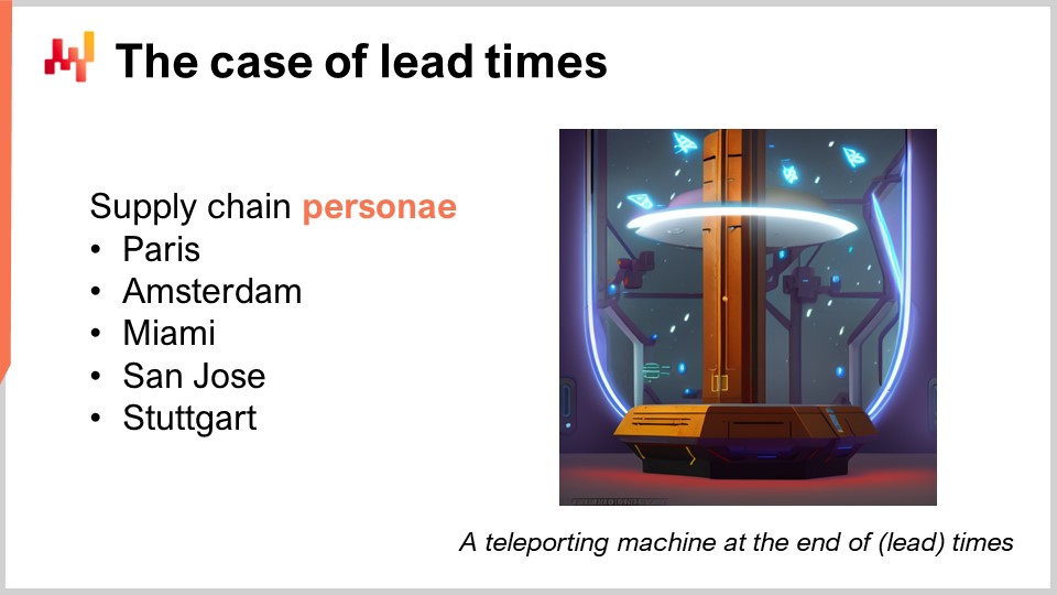
Thus, as a rough estimate, we have about a thousand times more papers about forecasting demand than there are about forecasting lead time. Supply chain books and supply chain software follow suit, leaving lead time as a second-class citizen and as an inconsequential technicality. However, the supply chain personnel that have been introduced in this series of lectures tell a different story. These personnel might represent fictitious companies, but they reflect supply chain archetypes. They tell us about the sort of situation that should be considered as typical. Let’s see what these personnel tell us as far as lead times are concerned.
Paris is a fictitious fashion brand operating its own retail network. Paris orders from overseas suppliers, with lead times being long and sometimes higher than six months. These lead times are only imperfectly known, and yet the new collection must hit the store at the right time as defined by the marketing operation associated with the new collection. The suppliers’ lead times require proper anticipation; in other words, they require a forecast.
Amsterdam is a fictitious FMCG company that specializes in the production of cheeses, creams, and butter. The ripening process of cheese is known and controlled, but it varies, with deviations of a few days. Yet, a few days is precisely the duration of the intense promotions triggered by the retail chains that happen to be the primary sales channel of Amsterdam. These manufacturing lead times require a forecast.
Miami is a fictitious aviation MRO. MRO stands for maintenance, repair, and overhaul. Every jetliner needs thousands of parts on a yearly basis to keep flying. A single missing part is likely to ground the aircraft. The repair duration for a repairable part, also referred to as TAT (turnaround time), defines when the rotable part becomes serviceable again. Yet, the TAT varies from days to months, depending on the extent of the repairs, which aren’t known at the time the part is removed from the aircraft. These TATs require a forecast.
San Jose is a fictitious e-commerce company that distributes a variety of home furnishings and accessories. As part of its service, San Jose provides a commitment for a delivery date for every transaction. However, the delivery itself depends on third-party companies that are far from being perfectly reliable. Thus, San Jose requires an educated guess about the delivery date that can be promised for every transaction. This educated guess is implicitly a lead time forecast.
Finally, Stuttgart is a fictitious automotive aftermarket company. It operates branches delivering car repairs. The lowest purchase price for the car parts can be obtained from wholesalers that offer long and somewhat irregular lead times. There are more reliable suppliers that are more expensive and closer. Choosing the right supplier for every part requires a proper comparative analysis of the respective lead times associated with various suppliers.
As we can see, every single supply chain personnel presented so far requires the anticipation of at least one, and frequently several, lead times. While it could be argued that forecasting demand requires more attention and effort than forecasting lead times, in the end, both are needed for nearly all supply chain situations.
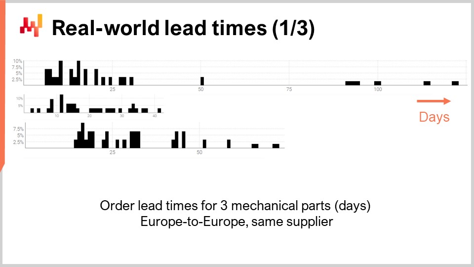
Thus, let’s have a look at a few actual real-world lead times. On the screen are three histograms that have been plotted by compiling observed lead times associated with three mechanical parts. These parts are ordered from the same supplier located in Western Europe. The orders come from a company also located in Western Europe. The x-axis indicates the duration of the observed lead times expressed in days, and the y-axis indicates the number of observations expressed as a percentage. In the following, all the histograms will adopt the same conventions, with the x-axis associated with durations expressed in days and the y-axis reflecting the frequency. From these three distributions, we can already make a few observations.
First, the data is sparse. We only have a few dozen data points, and these observations have been collected over several years. This situation is typical; if the company orders only once a month, it takes almost a decade to collect over 100 observations of lead times. Thus, whatever we do in terms of statistics, it should be geared towards small numbers rather than large numbers. Indeed, we will rarely get the luxury of dealing with large numbers.
Second, the lead times are erratic. We have observations ranging from a few days to a quarter. While it is always possible to compute an average lead time, relying on any kind of average value for any of those parts would be unwise. It is also clear that none of those distributions is even remotely normal.
Third, we have three parts that are somewhat comparable in size and price, and yet lead times vary a lot. While it might be tempting to lump together those observations to make the data less sparse, it is obviously unwise to do so, as it would be mixing distributions that are highly dissimilar. Those distributions don’t have the same mean, median, or even the same minimum or maximum.
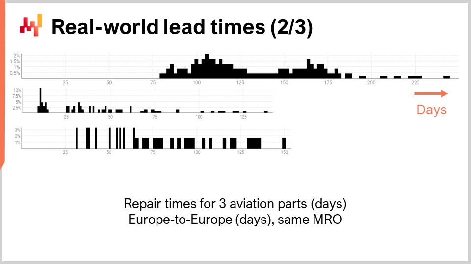
Let’s have a look at a second batch of lead times. These durations reflect the time it takes to repair three distinct aircraft parts. The first distribution appears to have two modes plus a tail. When a distribution presents two modes, it usually hints at the existence of a hidden variable that explains those two modes. For example, there might be two distinct types of repair operations, each type being associated with a lead time of its own. The second distribution appears to have one mode plus a tail. This mode matches a relatively short duration, about two weeks. It might reflect a process where the part gets inspected first, and sometimes the part is deemed serviceable without any further intervention, hence a much shorter lead time. The third distribution appears to be fully spread, without an obvious mode or tail. There might be multiple repair processes at play here that get lumped together. The sparsity of the data, with only three dozen observations, makes it difficult to say more. We will be revisiting this third distribution later in this lecture.
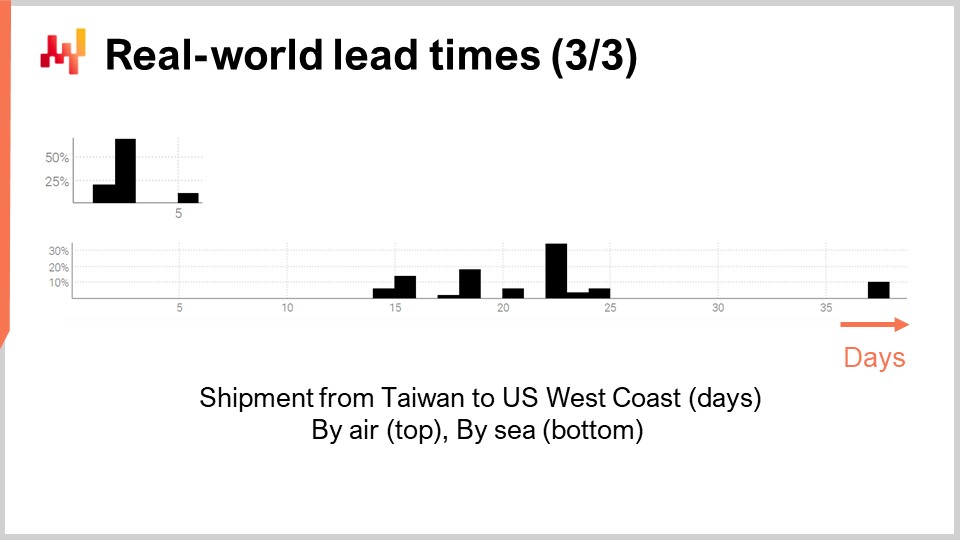
Finally, let’s have a look at two lead times reflecting the shipping delays from Taiwan to the US West Coast, either by air or by sea. Unsurprisingly, cargo aircraft are faster than cargo ships. The second distribution seems to hint that sometimes a sea shipment might miss its original ship and then get shipped with the next ship, almost doubling the delay. The very same phenomenon might be at play with the air shipment, although the data is so limited that it’s only a wild guess. Let’s point out that having access to only a couple of observations isn’t out of the ordinary as far as lead times are concerned. These situations are frequent. It is important to keep in mind that in this lecture, we are seeking tools and instruments that let us work with the lead time data we have, down to a handful of observations, not the lead time data we wish to have, like thousands of observations. The short gaps in both distributions also suggest a day-of-week cyclical pattern at work, although the present histogram visualization is not appropriate to validate this hypothesis.
From this short review of real-world lead times, we can already grasp some of the underlying phenomena that are at play. Indeed, lead times are highly structured; delays do not happen without cause, and those causes can be identified, decomposed, and quantified. However, the fine print of the lead time decomposition is frequently not recorded in the IT systems, at least not yet. Even when an extensive decomposition of the observed lead time is available, as it might be the case in certain industries like aviation, it does not imply that lead times can be perfectly anticipated. Sub-segments or phases within the lead time are likely to exhibit their own irreducible uncertainty.

This series of supply chain lectures presents my views and insights both on the study and on the practice of supply chain. I’m trying to keep these lectures somewhat independent, but they make more sense when being watched in sequence. The rest of this lecture depends on elements that have been previously introduced in this series, although I will be providing a refresher in a minute.
The first chapter is a general introduction to the field and study of supply chain. It clarifies the perspective that goes into this series of lectures. As you might have surmised already, this perspective diverges substantially from what would be considered the mainstream perspective on supply chain.
The second chapter introduces a series of methodologies. Indeed, supply chain defeats naive methodologies. Supply chains are made up of people who have agendas of their own; there is no such thing as a neutral party in supply chain. This chapter addresses those complications, including my own conflict of interest as the CEO of Lokad, an enterprise software company that specializes in predictive supply chain optimization.
The third chapter surveys a series of supply chain “personas.” These personas are fictitious companies that we have reviewed briefly today, and they are intended to represent archetypes of supply chain situations. The purpose of these personas is to focus exclusively on the problems, postponing the presentation of solutions.
The fourth chapter reviews the auxiliary sciences of supply chain. These sciences are not about supply chain per se, but they should be considered essential for a modern practice of supply chain. This chapter includes a progression through the abstraction layers, starting from computing hardware up to cybersecurity concerns.
The fifth and present chapter is dedicated to predictive modeling. Predictive modeling is a more general perspective than forecasting; it’s not just about forecasting demand. It’s about the design of models that can be used to estimate and quantify future factors of the supply chain of interest. Today, we delve into lead times, but more generally in supply chain, anything that isn’t known with a reasonable degree of certainty deserves a forecast.
The sixth chapter explains how optimized decisions can be computed while leveraging predictive models, and more specifically, probabilistic models that were introduced in the fifth chapter. The seventh chapter goes back to a largely non-technical perspective in order to discuss the actual corporate execution of a quantitative supply chain initiative.

Today, we focus on lead times. We have just seen why lead times matter, and we have just reviewed a short series of real-world lead times. Thus, we will proceed with elements of lead time modeling. As I will be adopting a probabilistic perspective, I will be briefly reintroducing the Continuous Rank Probability Score (CRPS), a metric to assess the goodness of a probabilistic forecast. I will also be introducing cross-validation and a variant of cross-validation that is suitable for our probabilistic perspective. With those tools in hand, we will introduce and assess our first non-naive probabilistic model for lead times. Lead time data are sparse, and the first item on our agenda is to smooth those distributions. Lead times can be decomposed into a series of intermediate phases. Thus, assuming that some decomposed lead time data are available, we need something to recompose those lead times while preserving the probabilistic angle.
Then, we will be reintroducing differentiable programming. Differentiable programming has already been used in this series of lectures to forecast demand, but it can be used to forecast lead times as well. We will do so, starting with a simple example intended to capture the impact of the Chinese New Year on lead times, a typical pattern observed when importing goods from Asia.
We will then proceed with a parametric probabilistic model for lead times, leveraging the log-logistic distribution. Again, differentiable programming will be instrumental in learning the parameters of the model. We will then extend this model by considering incomplete lead time observations. Indeed, even purchase orders that are not completed yet give us some information about the lead time.
Finally, we bring together a probabilistic lead time forecast and a probabilistic demand forecast within a single inventory replenishment situation. This will be the opportunity to demonstrate why modularity is an essential concern when it comes to predictive modeling, more important even than the fine print of the models themselves.
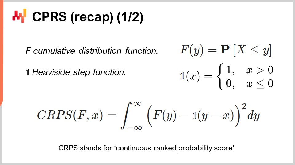
In Lecture 5.2 about probabilistic forecasting, we have already introduced some tools to assess the quality of a probabilistic forecast. Indeed, the usual accuracy metrics like mean square error or mean absolute error only apply to point forecasts, not probabilistic forecasts. Yet, it’s not because our forecasts become probabilistic that accuracy in the general sense becomes irrelevant. We just need a statistical instrument that happens to be compatible with the probabilistic perspective.
Among those instruments, there is the Continuous Rank Probability Score (CRPS). The formula is given on the screen. The CRPS is a generalization of the L1 metric, that is, the absolute error, but for probability distributions. The usual flavor of the CRPS compares a distribution, named F here, with an observation, named X here. The value obtained from the CRPS function is homogeneous with the observation. For example, if X is a lead time expressed in days, then the CRPS value is also expressed in days.
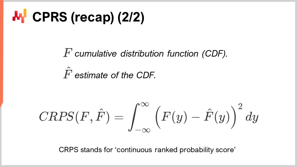
The CRPS can be generalized for the comparison of two distributions. This is what is being done on the screen. It’s just a minor variation of the previous formula. The essence of this metric remains unchanged. If F is the true lead time distribution and F_hat is an estimate of the lead time distribution, then the CRPS is expressed in days. The CRPS reflects the amount of difference between the two distributions. The CRPS can also be interpreted as the minimal amount of energy it takes to transport all the mass from the first distribution so that it takes the exact shape of the second distribution.
We now have an instrument to compare two one-dimensional probability distributions. This will become of interest in a minute as we introduce our first probabilistic model for lead times.
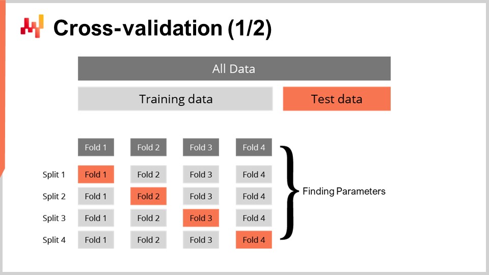
Having a metric to measure the goodness of a probabilistic forecast isn’t quite sufficient. The metric measures the goodness on the data we have; however, what we truly want is to be able to assess the goodness of our forecast under data that we don’t have. Indeed, it’s the future lead times that are of interest to us, not the lead times that have been already observed in the past. Our capacity to model for a model to perform well on the data that we don’t have is called generalization. Cross-validation is a general model validation technique precisely intended to assess the capacity of a model to generalize well.
In its simplest form, cross-validation consists of partitioning the observations into a small number of subsets. For each iteration, one subset is put aside and referred to as the test subset. The model is then generated or trained based on the other data subsets, referred to as the training subsets. After training, the model is validated against the test subset. This process is repeated a certain number of times, and the average goodness obtained over all the iterations represents the final cross-validated result.
Cross-validation is rarely used in the context of time series forecasting due to the time dependence between observations. Indeed, cross-validation, as just presented, assumes that the observations are independent. When time series are involved, backtesting is used instead. Backtesting can be seen as a form of cross-validation that takes time dependence into account.
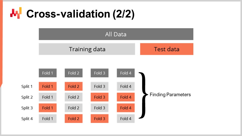
The cross-validation technique comes with numerous variants that reflect a vast array of potential angles that may need to be addressed. We will not be surveying those variants for the purpose of this lecture. I will be using a specific variant where, at every split, the training subset and the test subset have roughly the same size. This variant is introduced to deal with the validation of a probabilistic model, as we will see with some code in a minute.
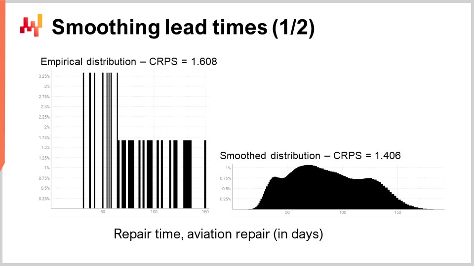
Let’s revisit one of the real-world lead times that we have previously seen on the screen. On the left, the histogram is associated with the third aviation repair time distributions. Those are the same observations as seen previously, and the histogram has merely been stretched vertically. By doing so, the two histograms on the left and on the right share the same scale. For the left histogram, we have about 30 observations. It’s not much, but it’s already more than what we will frequently get.
The histogram on the left is referred to as an empirical distribution. It’s literally the raw histogram as obtained from the observations. The histogram has one bucket for every duration expressed in an integral number of days. For every bucket, we count the number of observed lead times. Due to sparsity, the empirical distribution looks like a barcode.
There is a problem here. If we have two observed lead times at exactly 50 days, does it make sense to say that the probability of observing either 49 days or 51 days is exactly zero? It does not. Clearly, there is a spectrum of durations going on; we merely happen not to have enough data points to observe the real underlying distribution, which is most likely much smoother than this barcode-like distribution.
Thus, when it comes to smoothing this distribution, there is an indefinite number of ways to perform this smoothing operation. Some smoothing methods might look good but are not statistically sound. As a good starting point, we would like to ensure that a smooth model is more accurate than the empirical one. It turns out that we have already introduced two instruments, the CRPS and cross-validation, that will let us do that.
In a minute, the results are on display. The CRPS error associated with the barcode distribution is 1.6 days, while the CRPS error associated with the smooth distribution is 1.4 days. These two figures have been obtained through cross-validation. The lower error indicates that, in the sense of the CRPS, the distribution on the right is the most accurate one of the two. The difference of 0.2 between 1.4 and 1.6 is not that much; however, the key property here is that we have a smooth distribution that doesn’t erratically leave certain intermediate durations with a zero probability. This is reasonable, as our understanding of the repairs tells us that those durations would most likely end up happening if repairs are repeated. The CRPS doesn’t reflect the true depth of the improvement that we have just brought by smoothing the distribution. However, at the very least, lowering the CRPS confirms that this transformation is reasonable from a statistical perspective.
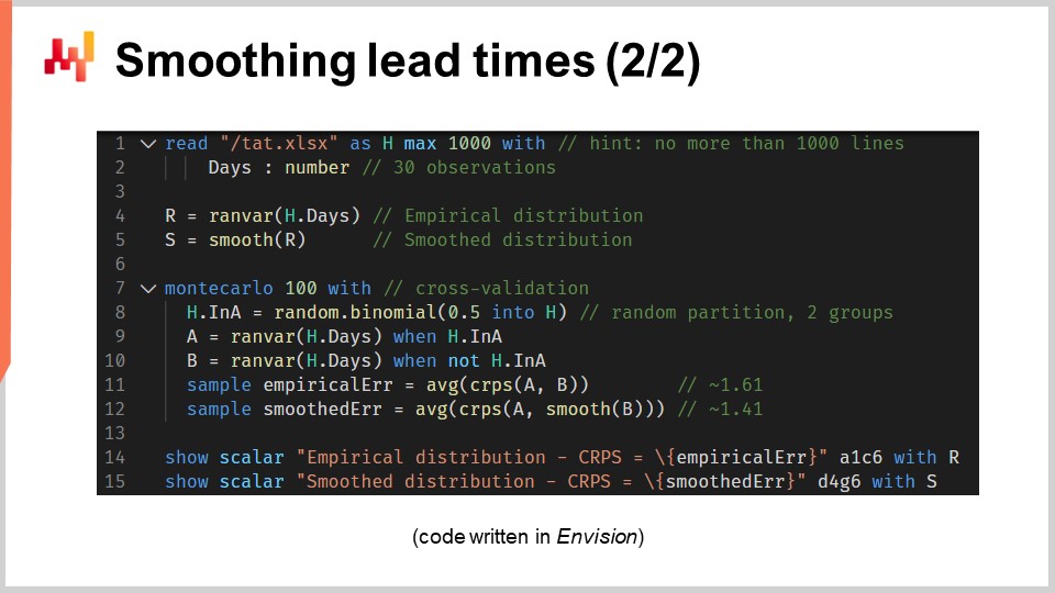
Let’s now have a look at the source code that has produced those two models and put those two histograms on display. All in all, this is achieved in 12 lines of code if we exclude the blank lines. As usual in this series of lectures, the code is written in Envision, the domain-specific programming language of Lokad dedicated to the predictive optimization of supply chains. However, there is no magic; this logic could have been written in Python. But for the sort of problems that we are considering in this lecture, Envision is more concise and more self-contained.
Let’s review those 12 lines of code. At lines 1 and 2, we are reading an Excel spreadsheet that has a single column of data. The spreadsheet contains 30 observations. This data is gathered within a table named “H” that has a single column named “days.” At line 4, we are building an empirical distribution. The variable “R” has the data type “ranvar,” and on the right side of the assignment, the “ranvar” function is an aggregator that takes observations as input and returns the histogram represented with a “ranvar” data type. As a result, the “ranvar” data type is dedicated to unidimensional integer distributions. We introduced the “ranvar” data type in a previous lecture of this chapter. This data type guarantees constant memory footprint and constant compute time for each operation. The downside of the “ranvar” as a data type is that a lossy compression is involved, although the data loss caused by the compression has been engineered to be inconsequential for supply chain purposes.
At line 5, we are smoothing the distribution with the built-in function named “smooth.” Under the hood, this function replaces the original distribution with a mixture of Poisson distributions. Each bucket of the histogram is transformed into a Poisson distribution with a mean equal to the integer position of the bucket, and finally, the mixture assigns a weight to each Poisson distribution proportional to the weight of the bucket itself. Another way to understand what this “smooth” function is doing is to consider that it’s equivalent to replacing every single observation by a Poisson distribution with a mean equal to the observation itself. All those Poisson distributions, one per observation, are then mixed. Mixing means averaging out the respective histogram bucket values. The “ranvar” variables “R” and “S” won’t be used again before lines 14 and 15, where they get displayed.
At line 7, we start a Monte Carlo block. This block is a sort of loop, and it’s going to be executed 100 times, as specified by the 100 values that appear right after the Monte Carlo keyword. The Monte Carlo block is intended to collect independent observations that are generated according to a process that involves a degree of randomness. You might be wondering why there is a specific Monte Carlo construct in Envision instead of just having a loop, as is usually the case with mainstream programming languages. It turns out that having a dedicated construct yields substantial benefits. First, it guarantees that the iterations are truly independent, down to the seeds used to derive the pseudorandomness. Second, it offers an explicit target for the automated distribution of the workload across several CPU cores or even across several machines.
At line 8, we create a random vector of Boolean values within the table “H.” With this line, we are creating independent random values, called deviates (true or false), for every line of the table “H.” As usual with Envision, the loops are abstracted away through array programming. With those Boolean values, we are partitioning the table “H” into two groups. This random split is used for the cross-validation process.
At lines 9 and 10, we are creating two “ranvars” named “A” and “B,” respectively. We are using the “ranvar” aggregator again, but this time, we are applying a filter with the “when” keyword just after the aggregator call. “A” is generated using only the lines where the value in “a” is true; for “B,” it’s the opposite. “B” is generated using only the lines where the value in “a” is false.
At lines 11 and 12, we collect the figures of interest from the Monte Carlo block. In Envision, the keyword “sample” can only be placed within a Monte Carlo block. It is used to collect the observations that are made while iterating many times through the Monte Carlo process. At line 11, we are computing the average error, expressed in CRPS terms, between two empirical distributions: a subsample from the original set of lead times. The “sample” keyword specifies that the values collected over the Monte Carlo iterations. The “AVG” aggregator, which stands for “average” on the right side of the assignment, is used to produce a single estimate at the end of the block.
At line 12, we do something almost identical to what happened at line 11. This time, however, we apply the “smooth” function to the “ranvar” “B.” We want to assess how close the smooth variant is from the naive empirical distribution. It turns out that it’s closer, at least in CRPS terms, than its original empirical counterparts.
At lines 14 and 15, we put the histograms and the CRPS values on display. Those lines generate the figures that we have seen in the previous slide. This script gives us our baseline for the quality of the empirical distribution of our model. Indeed, while this model, the “barcode” one, is arguably naive, it is a model nonetheless, and a probabilistic one at that. Thus, this script also gives us a better model, at least in the sense of the CRPS, through a smooth variant of the original empirical distribution.
Right now, depending on your familiarity with programming languages, it may seem like a lot to digest. However, I would like to point out how straightforward it is to produce a reasonable probability distribution, even when we don’t have more than a few observations. While we have 12 lines of code, only lines 4 and 5 represent the true modeling part of the exercise. If we were only interested in the smooth variant, then the “ranvar” “S” could be written with a single line of code. Thus, it’s literally a one-liner in terms of code: first, apply a ranvar aggregation, and second, apply a smooth operator, and we are done. The rest is just instrumentation and display. With the proper tools, probabilistic modeling, whether it be lead time or something else, can be made extremely straightforward. There is no grand mathematics involved, no grand algorithm, no grand software pieces. It is simple and remarkably so.
How do you get a shipment six months late? The answer is obvious: one day at a time. More seriously, lead times can usually be decomposed into a series of delays. For example, a supplier lead time can be decomposed into a waiting delay as the order is put into a backlog queue, followed by a manufacturing delay as goods get produced, and finally followed by a transit delay as goods get shipped. Thus, if lead times can be decomposed, it is also of interest to be able to recompose them.
If we were to live in a highly deterministic world where the future could be precisely anticipated, then recomposing lead times would be just a matter of playing addition. Going back to the example I just mentioned, composing the ordering lead time would be the sum of the queuing delay in days, the manufacturing delay in days, and the transit delay in days. Yet, we do not live in a world where the future can be precisely anticipated. The real-world lead time distributions that we presented at the beginning of this lecture support this proposition. Lead times are erratic, and there is little reason to believe that this will fundamentally change in the coming decades.
Thus, future lead times should be approached as random variables. These random variables embrace and quantify the uncertainty instead of dismissing it. More specifically, this means that each component of the lead time should also be individually modeled as a random variable. Going back to our example, the ordering lead time is a random variable, and it is obtained as the sum of three random variables respectively associated with the queuing delay, the manufacturing delay, and the transit delay.
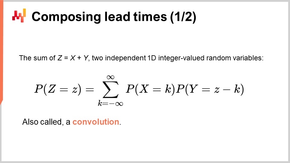
The formula for the sum of two independent, one-dimensional, integer-valued random variables is presented on the screen. This formula merely states that if we get a total duration of Z days, and if we have K days for the first random variable X, then we must have Z minus K days for the second random variable Y. This type of summation is known, generally speaking, in mathematics as convolutions.
While it seems that there is an infinite number of terms in this convolution, in practice, we only care about a finite number of terms. First, all the negative durations have a zero probability; indeed, negative delays would mean traveling back in time. Second, for large delays, probabilities become so small that for practical supply chain purposes, they can reliably be approximated as zeros.
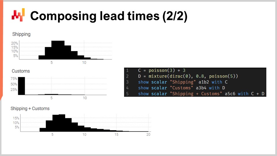
Let’s put these convolutions into practice. Let’s consider a transit time that can be decomposed into two phases: a shipping delay followed by a clearance delay at customs. We want to model these two phases with two independent random variables and then recompose the transit time by adding those two random variables.
On the screen, the histograms on the left are produced by the script on the right. At line 1, the shipping delay is modeled as a convolution of a Poisson distribution plus a constant. The Poisson function returns a “ranvar” data type; adding three has the effect of shifting the distribution to the right. The resulting “ranvar” is assigned to the variable “C.” This “ranvar” is put on display at line 3. It can be seen on the left as the topmost histogram. We recognize the shape of a Poisson distribution that has been shifted to the right by a few units, three units in this case. At line two, the custom clearance is modeled as a mixture of a Dirac at zero and a Poisson at five. The Dirac at zero occurs eighty percent of the time; that’s what this 0.8 constant means. It reflects situations where most of the time, goods are not even inspected by customs and go through without any notable delay. Alternatively, twenty percent of the time, the goods are inspected at customs, and the delay is modeled as a Poisson distribution with a mean of five. The resulting ranvar is assigned to a variable named D. This ranvar is put on display at line four and can be seen on the left as the middle histogram. This asymmetrical aspect reflects that most of the time, customs do not add any delay.
Finally, at line five, we compute C plus D. This addition is a convolution, as both C and D are ranvars, not numbers. This is the second convolution in this script, as a convolution already took place at line one. The resulting ranvar is put on display and is visible on the left as the third and lowest histogram. This third histogram is similar to the first one, except that the tail is spreading much further to the right. Once again, we see that with a few lines of code, we can approach non-trivial real-world effects, such as clearance delays at customs.
However, two criticisms could be made about this example. First, it doesn’t say where the constants come from; in practice, we want to learn those constants from historical data. Second, while the Poisson distribution has the advantage of simplicity, it might not be a very realistic shape for lead time modeling, especially considering fat-tail situations. Thus, we are going to address those two points in order.
To learn parameters from data, we are going to revisit a programming paradigm that we have already introduced in this series of lectures, namely differentiable programming. If you haven’t watched the previous lectures in this chapter, I invite you to have a look at them after the end of the present lecture. Differentiable programming is introduced in greater detail in those lectures.
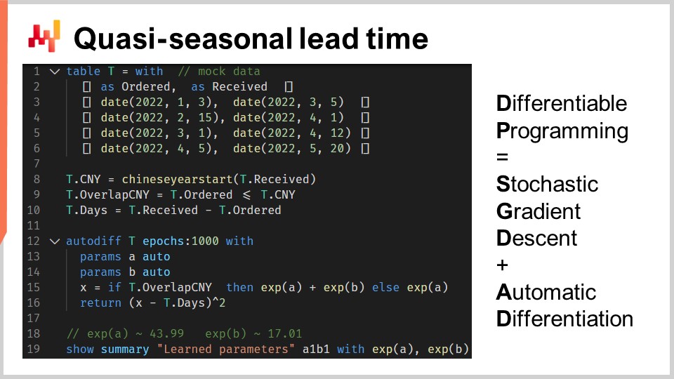
Differentiable programming is a combination of two techniques: stochastic gradient descent and automatic differentiation. Stochastic gradient descent is an optimization technique that nudges the parameters one observation at a time in the opposite direction of the gradients. Automatic differentiation is a compilation technique, as in the compiler of a programming language; it computes the gradients for all the parameters that appear within a general program.
Let’s illustrate differentiable programming with a lead time problem. This will serve either as a refresher or as an introduction, depending on your familiarity with this paradigm. We want to model the impact of the Chinese New Year on lead times associated with imports from China. Indeed, as factories close for two or three weeks for the Chinese New Year, lead times get longer. The Chinese New Year is cyclical; it happens every year. However, it is not strictly seasonal, at least not in the sense of the Gregorian calendar.
At lines one to six, we are introducing some mock purchase orders with four observations, with both an order date and a received date. In practice, this data would not be hard-coded, but we would load this historical data from the company’s systems. At lines eight and nine, we compute whether the lead time overlaps with the Chinese New Year. The variable “T.overlap_CNY” is a Boolean vector; it indicates whether the observation is impacted by the Chinese New Year or not.
At line 12, we introduce an “autodiff” block. The table T is used as the observation table, and there are 1000 epochs. This means that each observation, so each line in the table T, is going to be visited a thousand times. One step of the stochastic gradient descent corresponds to one execution of the logic within the “autodiff” block.
At lines 13 and 14, two scalar parameters are declared. The “autodiff” block will learn these parameters. The parameter A reflects the baseline lead time without the Chinese New Year effect, and the parameter B reflects the extra delay associated with the Chinese New Year. At line 15, we compute X, the lead time prediction of our model. This is a deterministic model, not a probabilistic one; X is a point lead time forecast. The right side of the assignment is straightforward: if the observation overlaps the Chinese New Year, then we return the baseline plus the New Year component; otherwise, we only return the baseline. As the “autodiff” block takes only a single observation at a time, at line 15, the variable T.overlap_CNY refers to a scalar value and not to a vector. This value matches the one line picked as the observation line within the table T.
The parameters A and B are wrapped into the exponential function “exp,” which is a small differentiable programming trick. Indeed, the algorithm that pilots the stochastic gradient descent tends to be relatively conservative when it comes to the incremental variations of the parameters. Thus, if we want to learn a positive parameter that may grow larger than, say, 10, then wrapping this parameter into an exponential process speeds up the convergence.
At line 16, we return a mean square error between our prediction X and the observed duration, expressed in days (T.days). Again, inside this “autodiff” block, T.days is a scalar value and not a vector. As the table T is used as the observation table, the return value is treated as the loss that gets minimized through the stochastic gradient descent. The automatic differentiation propagates the gradients from the loss backward to the parameters A and B. Finally, at line 19, we display the two values that we have learned, respectively, for A and B, which are the baseline and the New Year component of our lead time.
This concludes our reintroduction of differentiable programming as a versatile tool that learns statistical patterns. From here, we’ll be revisiting the “autodiff” blocks with more elaborate situations. However, let’s point out once more that even if it may feel a little overwhelming, there is nothing really complicated going on here. Arguably, the most complicated piece of code in this script is the underlying implementation of the function “ChineseYearStart,” called at line eight, which happens to be part of the Envision standard library. Within a few lines of code, we introduce a model with two parameters and learn those parameters. Once again, this simplicity is remarkable.
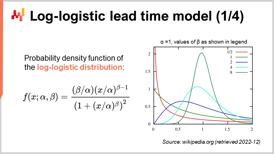
Lead times are frequently fat-tailed; that is, when a lead time deviates, it deviates by a lot. Thus, in order to model lead time, it is of interest to adopt distributions that can reproduce those fat-tail behaviors. The mathematical literature presents an extensive list of such distributions, and quite a few would suit our purpose. However, merely surveying the mathematical landscape would take us hours. Let’s just point out that the Poisson distribution does not have a fat tail. Thus, today, I will be picking the log-logistic distribution, which happens to be a fat-tail distribution. The primary justification for this choice of distribution is that the Lokad teams are modeling lead times through log-logistic distributions for several clients. It happens to be working well with a minimum number of complications. Let’s keep in mind, however, that the log-logistic distribution is in no way a silver bullet, and there are numerous situations where Lokad models lead times differently.
On the screen, we have the probability density function of the log-logistic distribution. This is a parametric distribution that depends on two parameters, alpha and beta. The alpha parameter is the median of the distribution, and the beta parameter governs the shape of the distribution. On the right, a short series of shapes can be obtained through various beta values. While this density formula may look intimidating, it is literally textbook material, just like the formula to compute the volume of a sphere. You may try to decipher and memorize this formula, but it’s not even necessary; you just need to know that an analytical formula exists. Once you know that the formula exists, finding it back online takes less than a minute.
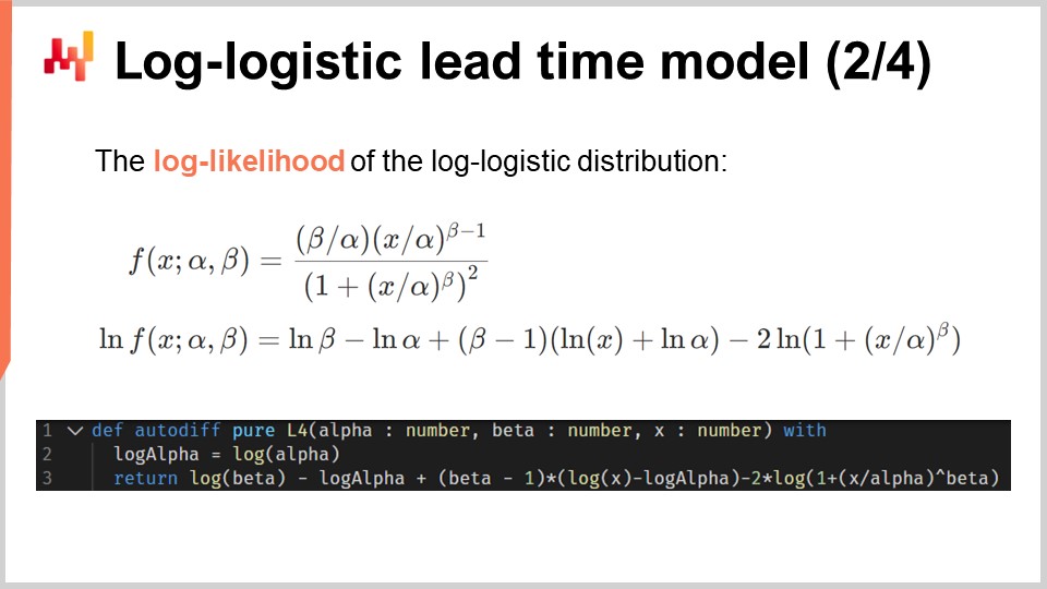
Our intent is to leverage the log-logistic distribution to learn a probabilistic lead time model. In order to do this, we are going to minimize the log-likelihood. Indeed, in the previous lecture within this fifth chapter, we have seen that there are several metrics that are appropriate for the probabilistic perspective. A little while ago, we revisited the CRPS (Continuous Ranked Probability Score). Here, we revisit the log-likelihood, which adopts a Bayesian perspective.
In a nutshell, given two parameters, the log-logistic distribution tells us the probability to observe each observation as found in the empirical dataset. We want to learn the parameters that maximize this likelihood. The logarithm, hence the log-likelihood rather than the plain likelihood, is introduced to avoid numerical underflows. Numerical underflows happen when we process very small numbers, very close to zero; those very small numbers don’t play well with the floating-point representation as commonly found in modern computing hardware.
Thus, in order to compute the log-likelihood of the log-logistic distribution, we apply the logarithm to its probability density function. The analytical expression is given on the screen. This expression can be implemented, and this is exactly what is done in the three lines of code below.
At line one, the function “L4” is introduced. L4 stands for “log-likelihood of log-logistic” – yes, that’s a lot of L’s and a lot of logs. This function takes three arguments: the two parameters alpha and beta, plus the observation x. This function returns the logarithm of the likelihood. The function L4 is decorated with the keyword “autodiff”; the keyword indicates that this function is intended to be differentiated through automatic differentiation. In other words, gradients can flow backward from the return value of this function back to its arguments, the parameters alpha and beta. Technically, the gradient flows backward through the observation x as well; however, as we will keep the observations immutable during the learning process, the gradients won’t have any effect on the observations. At line three, we get the literal transcription of the mathematical formula just above the script.
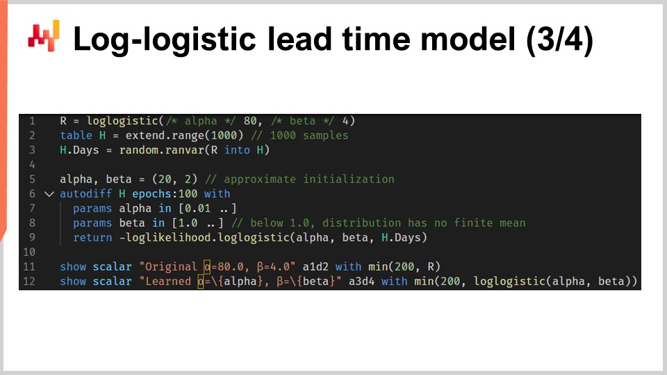
Let’s now put things together with a script that learns the parameters of a probabilistic lead time model based on the log-logistic distribution. In lines one and three, we generate our mock training dataset. In real-world settings, we would be using historical data instead of generating mock data. At line one, we create a “ranvar” that represents the original distribution. For the sake of the exercise, we want to learn back those parameters, alpha and beta. The log-logistic function is part of the standard library of Envision and it returns a “ranvar”. At line two, we create the table “H”, which contains 1,000 entries. At line three, we draw 1,000 deviates that are randomly sampled from the original distribution “R”. This vector “H.days” represents the training dataset.
At line six, we have an “autodiff” block; this is where the learning takes place. At lines seven and eight, we declare two parameters, alpha and beta, and in order to avoid numerical problems like division by zero, bounds are applied to those parameters. Alpha must remain greater than 0.01 and beta must remain greater than 1.0. At line nine, we return the loss, which is the opposite of the log-likelihood. Indeed, by convention, “autodiff” blocks minimize the loss function, and thus we want to maximize the likelihood, hence the minus sign. The function “log_likelihood.logistic” is part of the standard library of Envision, but under the hood, it is just the function “L4” that we have implemented in the previous slide. Thus, there is no magic at play here; it is all automated differentiation that makes the gradient flow backward from the loss to the parameters alpha and beta.
At lines 11 and 12, the original distribution and the learned distribution are plotted. The histograms are capped at 200; this cap makes the histogram a little bit more readable. We will get back to that in a minute. In case you are wondering about the performance of the “autodiff” portion of this script, it takes under 80 milliseconds to execute on a single CPU core. Differentiable programming isn’t just versatile; it also makes good use of the computing resources provided by modern computing hardware.
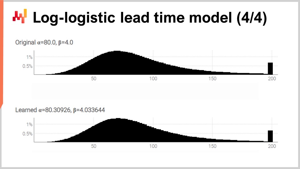
On the screen, we have the two histograms produced by our script that we have just reviewed. On top, the original distribution with its two original parameters, alpha and beta, at 80 and 4, respectively. At the bottom, the learned distribution with two parameters learned through differentiable programming. Those two spikes on the far right are associated with the tails that we have truncated, as those tails extend quite far. By the way, while it is rare, it does happen for certain goods to be received more than one year after they were ordered. This is not the case for every vertical, certainly not for dairy, but for mechanical parts or electronics, it does happen occasionally.
While the learning process isn’t exact, we get results within one percent of the original parameter values. This demonstrates, at the very least, that this log-likelihood maximization through differentiable programming does work in practice. The log-logistic distribution may or may not be appropriate; it depends on the shape of the lead time distribution that you are facing. However, we can pretty much pick any alternative parametric distribution. All it takes is an analytical expression of the probability density function. There is a vast array of such distributions. Once you have a textbook formula, a straightforward implementation through differentiable programming usually does the rest.
Lead times are not just observed once the transaction is final. While the transaction is still in progress, you already know something; you already have an incomplete lead time observation. Let’s consider that 100 days ago, you placed an order. The goods haven’t been received yet; however, you already know that the lead time is at least 100 days. This duration of 100 days represents the lower bound for a lead time that has yet to be observed completely. Those incomplete lead times are frequently quite important. As I mentioned at the beginning of this lecture, lead time datasets are frequently sparse. It’s not unusual to have a dataset that only includes half a dozen observations. In those situations, it is important to make the most of every observation, including the ones that are still in progress.
Let’s consider the following example: we have five orders in total. Three orders have already been delivered with lead time values that were very close to 30 days. However, the last two orders have been pending for 40 days and 50 days, respectively. According to the first three observations, the average lead time should be around 30 days. However, the last two orders that are still incomplete disprove this hypothesis. The two pending orders at 40 and 50 days hint at a lead time substantially longer. Thus, we should not discard the last orders just because they are incomplete. We should leverage this information and update our belief toward longer lead times, maybe 60 days.
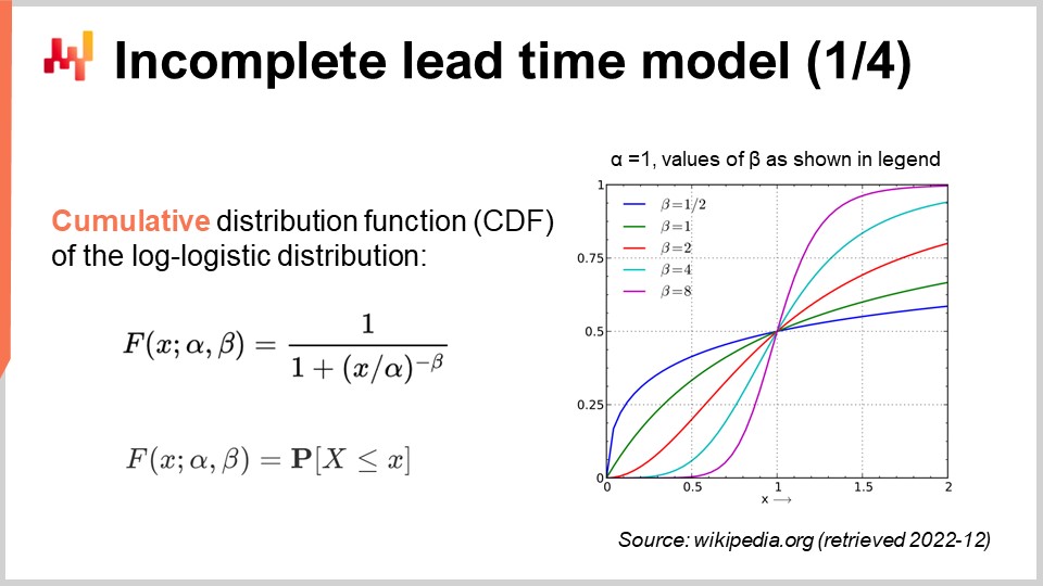
Let’s revisit our probabilistic lead time model, but this time, take incomplete observations into account. In other words, we want to deal with observations that are sometimes just a lower bound for the final lead time. In order to do that, we can use the cumulative distribution function (CDF) of the log-logistic distribution. This formula is written on the screen; again, this is textbook material. The CDF of the log-logistic distribution happens to benefit from a simple analytical expression. In the following, I will be referring to this technique as the “conditional probability technique” to deal with censored data.
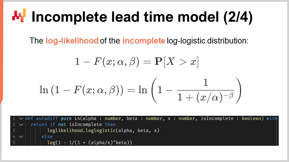
Based on this analytical expression of the CDF, we can revisit the log-likelihood of the log-logistic distribution. The script on the screen provides a revised implementation of our previous L4 implementation. At line one, we have pretty much the same function declaration. This function takes an extra fourth argument, a Boolean value named “is_incomplete” that indicates, as the name suggests, whether the observation is incomplete or not. At lines two and three, if the observation is complete, then we fall back to the previous situation with the regular log-logistic distribution. Thus, we call the log-likelihood function that is part of the standard library. I could have repeated the code of the previous L4 implementation, but this version is more concise. At lines four and five, we express the log-likelihood of ultimately observing a lead time greater than the current incomplete observation, “X”. This is achieved through the CDF and, more precisely, the logarithm of the CDF.
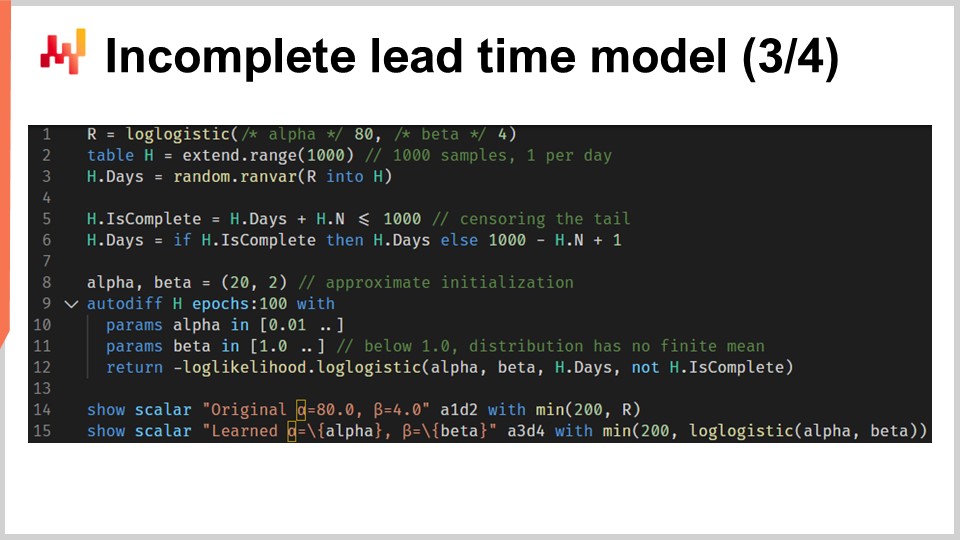
We can now repeat our setup with a script that learns the parameters of the log-logistic distribution, but this time in the presence of incomplete lead times. The script on the screen is almost identical to the previous one. At lines one to three, we generate the data; these lines have not changed. Let’s point out that H.N is an auto-generated vector that is implicitly created at line two. This vector numbers the generated lines, starting at one. The previous version of this script wasn’t using this auto-generated vector, but presently, the H.N vector does appear at the end of line six.
Lines five and six are indeed the important ones. Here, we censor the lead times. It is as if we were making one lead time observation per day and truncating the observations that are too recent to be informed. This means, for example, that a 20-day lead time initiated seven days ago appears as a seven-day incomplete lead time. By the end of line six, we have generated a list of lead times where some of the recent observations (the ones that would terminate beyond the present date) are incomplete. The rest of the script is unchanged, except for line 12, where the H.is_complete vector is passed as the fourth argument of the log-likelihood function. Thus, we are calling, at line 12, the differentiable programming function that we just introduced a minute ago.
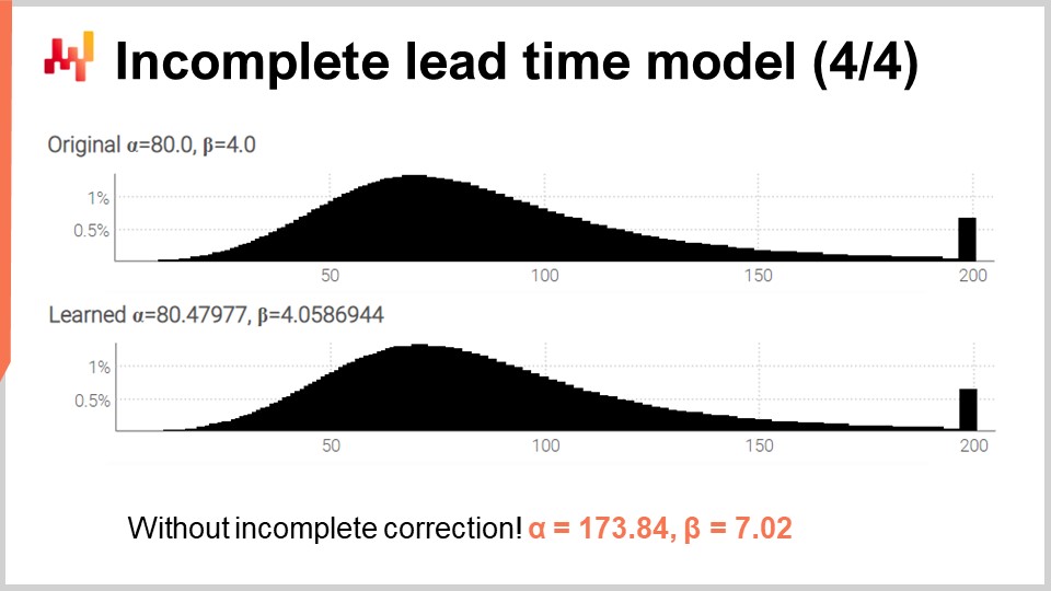
Finally, on the screen, the two histograms are produced by this revised script. The parameters are still learned with high accuracy, while we are now in the presence of numerous incomplete lead times. In order to validate that dealing with incomplete times wasn’t an unnecessary complication, I’ve re-executed the script, but this time with a modified variation with the three-argument overload of the log-likelihood function (the one that we used initially and assumed that all the observations are complete). For alpha and beta, we get the values displayed at the bottom of the screen. As expected, those values do not match at all the original values of alpha and beta.
In this series of lectures, this is not the first time that a technique has been introduced to deal with censored data. In the second lecture of this chapter, the loss masking technique has been introduced to deal with stockouts. Indeed, we typically want to predict future demand, not future sales. Stockouts introduce a downward bias, as we don’t get to observe all the sales that would have happened if the stockout hadn’t occurred. The conditional probability technique can be used to deal with censored demand as it happens with stockouts. The conditional probability technique is a bit more complex than loss masking, so it should probably not be used if loss masking is enough.
In the case of lead times, data sparsity is the primary motivation. We may have so little data that it may be critical to make the most of every single observation, even the incomplete ones. Indeed, the conditional probability technique is more powerful than loss masking in the sense that it does leverage incomplete observations instead of just discarding them. For example, if there is one unit in stock and if this one unit in stock gets sold, then, hinting at a stockout, the conditional probability technique still makes use of the information that the demand was greater or equal to one.
Here, we get a surprising benefit of probabilistic modeling: it gives us a graceful way to deal with censorship, an effect that occurs in numerous supply chain situations. Through conditional probability, we can eliminate entire classes of systematic biases.
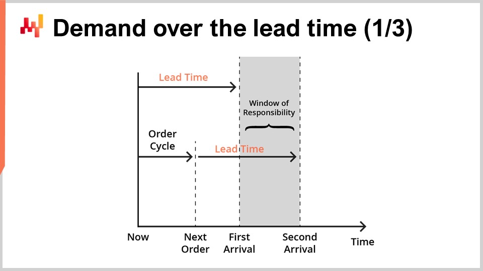
Lead time forecasts are typically intended to be combined with demand forecasts. Indeed, let’s now consider a simple inventory replenishment situation, as illustrated on the screen.
We serve a single product, and the stock can be replenished by reordering from a single supplier. We are seeking a forecast that would support our decision to reorder or not from the supplier. We can reorder now, and if we do so, the goods will arrive at the point in time noted as “first arrival.” Later, we will have another opportunity to reorder. This later opportunity happens at a point in time noted as “next order,” and in this case, the goods will arrive at the point in time noted as “second arrival.” The period indicated as the “window of responsibility” is the period that matters as far as our reorder decision is concerned.
Indeed, whatever we decide to reorder won’t arrive before the first lead time. Thus, we have already lost control over servicing the demand for anything that happens prior to the first arrival. Then, as we will get a later opportunity to reorder, servicing the demand after the second arrival isn’t our responsibility anymore; it’s the responsibility of the next reorder. Thus, reordering while intending to serve the demand beyond the second arrival should be postponed until the next reorder opportunity.
In order to support the reorder decision, there are two factors that should be forecasted. First, we should forecast the expected stock on hand at the time of the first arrival. Indeed, if by the time of the first arrival, there is still plenty of stock left, then there is no reason to reorder now. Second, we should forecast the expected demand for the duration of the window of responsibility. In a real setup, we would also have to forecast the demand beyond the window of responsibility in order to assess the carrying cost of the goods that we are ordering now, as there might be leftovers that spill into later periods. However, for the sake of concision and timing, we are going to focus today on the expected stock and the expected demand as far as the window of responsibility is concerned.
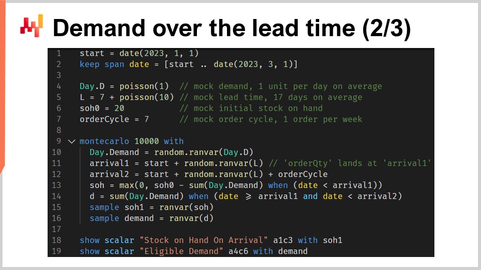
This script implements the window of responsibility factors or forecasts that we just discussed. It takes as input a probabilistic lead time forecast and a probabilistic demand forecast. It returns two distributions of probabilities, namely the stock at hand on arrival and the eligible demand as scoped by the window of responsibility.
At lines one and two, we set up the timelines, which start on January 1st and end on March 1st. In a prediction setup, this timeline would not be hardcoded. At line four, a simplistic probabilistic demand model is introduced: a Poisson distribution repeated day by day for the entire duration of this timeline. The demand will be one unit per day on average. I’m using here a simplistic model for the demand for the sake of clarity. In a real setup, we would, for example, use an ESSM (Ensemble State Space Model). State space models are probabilistic models, and they have been introduced in the very first lecture of this chapter.
At line five, another simplistic probabilistic model is introduced. This second model is intended for lead times. It’s a Poisson distribution shifted by seven days to the right. The shift is performed through a convolution. At line six, we define the initial stock at hand. At line seven, we define the order cycle. This value is expressed in days and characterizes when the next reorder will take place.
From line 9 to 16, we have a Monte Carlo block that represents the core logic of the script. Earlier in this lecture, we have already introduced another Monte Carlo block to support our cross-validation logic. Here, we are using this construct again, but for a different purpose. We want to compute two random variables reflecting, respectively, the stock in hand on arrival and the eligible demand. However, the algebra of random variables is not expressive enough to perform this calculation. Thus, we are using a Monte Carlo block instead.
In the third lecture of this chapter, I pointed out that there is a duality between probabilistic forecasting and simulations. The Monte Carlo block illustrates this duality. We start with a probabilistic forecast, turn it into a simulation, and finally, convert the results of the simulation back into another probabilistic forecast.
Let’s have a look at the fine print. At line 10, we generate one trajectory for the demand. At line 11, we generate the arrival date for the first order, assuming that we are ordering today. At line 12, we generate the arrival date for the second order, assuming that we are ordering one order cycle from now. At line 13, we compute what remains as stock on hand at the first arrival date. It is the initial stock at hand minus the demand observed for the duration of the first lead time. The max zero states that the stock can’t go into the negatives. In other words, we assume that we don’t take any backlog. This no backlog assumption could be modified. The backlog case is left as an exercise to the audience. As a hint, differentiable programming can be used to assess the percentage of the unserved demand that converts successfully into backlogs, depending on how many days there are before the renewed availability of the stock.
Back to the script, at line 14, we compute the eligible demand, which is the demand that happens during the window of responsibility. At lines 15 and 16, we collect two random variables of interest through the “sample” keyword. Unlike the first Envision script of this lecture, which dealt with cross-validation, we seek here to collect distributions of probabilities from this Monte Carlo block, not just averages. On both lines 15 and 16, the random variable that appears on the right side of the assignment is an aggregator. At line 15, we get a random variable for the stock in hand on arrival. At line 16, we get another random variable for the demand that happens within the window of responsibility.
At lines 18 and 19, those two random variables are put on display. Now, let’s pause for a second and reconsider this whole script. The lines one to seven are merely dedicated to the setup of the mock data. The lines 18 and 19 are just displaying the results. The only actual logic happens over the eight lines between lines 9 and 16. In fact, all the actual logic is located, in a sense, at lines 13 and 14.
With just a few lines of code, less than 10 no matter how we count, we combine a probabilistic lead time forecast with a probabilistic demand forecast in order to compose some sort of hybrid probabilistic forecast of actual supply chain significance. Let’s note that there is nothing here that really depends on the specifics of either the lead time forecast or the demand forecast. Simple models have been used, but sophisticated ones could have been used instead. It would not have changed anything. The only requirement is to have two probabilistic models so that it becomes possible to generate those trajectories.
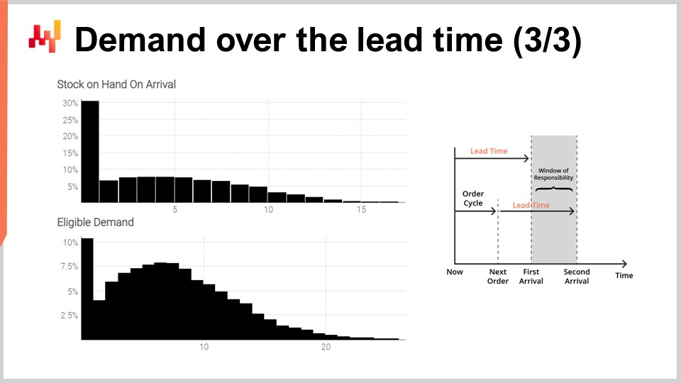
Finally, on the screen, the histograms as produced by the script. The top histogram represents the stock in hand on arrival. There is a 30% chance, roughly, to face an initial stock at zero. In other words, there is a 30% chance that a stock out may have happened by the last day just prior to the first arrival date. The average stock value might be something like five units. However, if we were to judge this situation by its average, we would be seriously misreading the situation. A probabilistic forecast is essential to properly reflect the initial stock situation.
The bottom histogram represents the demand associated with the window of responsibility. We have a 10% chance, roughly, of facing zero demand. This result might also be perceived as surprising. Indeed, we started this exercise with a stationary Poisson demand of one unit per day on average. We have seven days between orders. If it was not for the varying lead time, there should have been less than a 0.1% chance of getting zero demand over seven days. However, the script proves that this occurrence is much more frequent. The reason is that a small window of responsibility may happen if the first lead time is longer than usual and if the second lead time is shorter than usual.
Facing zero demand over the window of responsibility means that the stock in hand is likely to become quite high at a point in time. Depending on the situation, this might or might not be critical, but it might be, for example, if there is a stocking capacity limit or if the stock is perishable. Once again, the average demand, probably around eight, does not provide a reliable insight into what the demand looked like. Remember that we have obtained this highly asymmetrical distribution from an initial stationary demand, one unit per day on average. This is the varying lead time effect in action.
This simple setup demonstrates the importance of lead times when it comes to inventory replenishment situations. From a supply chain perspective, isolating lead time forecasts from demand forecasts is, at best, a practical abstraction. The daily demand is not what we are truly interested in. What is of true interest is the composition of the demand with the lead time. If other stochastic factors were present, like backlogs or returns, those factors would have been part of the model as well.

The present chapter in this series of lectures is titled “Predictive Modeling” instead of “Demand Forecasting,” as it would typically be the case in mainstream supply chain textbooks. The reason for this chapter title should have become progressively obvious as we progress through the present lecture. Indeed, from a supply chain perspective, we want to forecast the evolution of the supply chain system. Demand is certainly an important factor, but it’s not the only factor. Other varying factors like lead time must be forecast. Even more importantly, all those factors must be, in the end, forecast together.
Indeed, we need to bring those predictive components together to support a decision-making process. Thus, what matters is not seeking some sort of end game demand forecasting model. This task is largely a fool’s errand, ultimately, because the extra accuracy will be gained in ways that run contrary to the best interest of the company. More sophistication means more opacity, more bugs, more computing resources. As a rule of thumb, the more sophisticated the model, the harder it becomes to successfully operationally compose this model with another model. What matters is to assemble a collection of predictive techniques that can be composed at will. This is what modularity is about from a perspective of predictive modeling. In this lecture, half a dozen techniques have been presented. These techniques are useful as they address critical real-world angles like incomplete observations. They are simple as well; none of the code examples presented today exceeded 10 lines of actual logic. Most importantly, these techniques are modular, like Lego bricks. They work well together and can be almost endlessly recombined.
The end game of predictive modeling for supply chain, as it should be understood, is the identification of such techniques. Each technique should be, by itself, an opportunity to revisit any pre-existing predictive model in order to simplify or improve this model.
In conclusion, despite lead time being largely ignored by the academic community, lead time can and should be forecast. By reviewing a short series of real-world lead time distributions, we have identified two challenges: firstly, lead times vary; second, lead times are sparse. Thus, we have introduced modeling techniques that are appropriate to deal with lead time observations that happen to be both sparse and erratic.
These lead time models are probabilistic and are, to a large extent, the continuation of the models that have been gradually introduced through this chapter. We have also seen that the probability perspective does provide an elegant solution to the problem of incomplete observation, an almost ubiquitous aspect in supply chain. This problem occurs whenever there are stock outs and whenever there are pending orders. Finally, we have seen how to compose a probabilistic lead time forecast with a probabilistic demand forecast in order to craft the predictive model that we need to support a later decision-making process.
The next lecture will be on the 8th of March. It will be a Wednesday at the same time of the day, 3 PM Paris time. Today’s lecture was technical, but the next one will be largely non-technical, and I will be discussing the case of the supply chain scientist. Indeed, mainstream supply chain textbooks approach supply chain as if forecasting models and optimization models emerge and operate out of thin air, entirely ignoring their “wetware” component—that is, the people in charge. Thus, we will have a closer look at the roles and responsibilities of the supply chain scientist, a person who is expected to spearhead the quantitative supply chain initiative.
Now, I will be proceeding with the questions.
Question: What if someone wants to keep their stock for further innovation or for reasons other than just in time or other concepts?
This is indeed a very important question. The concept is typically addressed through the economic modeling of the supply chain, which we technically call the “economic drivers” in this series of lectures. What you’re asking is whether it’s better not to serve a customer today because, at a later point in time, there will be an opportunity to serve the same unit to another person that matters more for whatever reason. In essence, what you’re saying is that there is more value to be captured by serving another customer later, perhaps a VIP customer, than serving a customer today.
This might be the case, and it does happen. For example, in the aviation industry, let’s say you are an MRO (Maintenance, Repair, and Overhaul) provider. You have your usual VIP clients—the airlines that you routinely serve with long-term contracts, and they are very important. When this happens, you want to make sure that you will always be able to serve those clients. But what if another airline gives you a call and asks for one unit? In this case, what will happen is that you could serve this person, but you don’t have a long-term contract with them. So, what you’re going to do is adjust your price so that it’s very high, ensuring that you get enough value to make up for the potential stock out that you may face at a later point in time. Bottom line for this first question, I believe that it’s not really a matter of forecasting but more a matter of proper modeling of the economic drivers. If you want to preserve stock, what you want is to generate a model—an optimization model—where the rational response is not to serve the client asking for one unit while you still have stock in reserve.
By the way, another typical situation for that is when you’re selling kits. A kit is an assembly of many parts that is sold together, and you have just one part left that is worth only a small fraction of the total kit’s value. The problem is that if you sell this last unit, you can’t build your kit and sell it at its full price anymore. Thus, you might be in a situation where you prefer to keep the unit in stock just for the sake of being able to sell the kit at a later time, potentially with some uncertainty. But again, it boils down to the economic drivers, and that would be the way I would approach this situation.
Question: During the last few years, most supply chain delays happened because of war or pandemic, which is very difficult to forecast because we didn’t have such situations before. What is your take on this?
My take is that lead times have been varying forever. I’ve been in the supply chain world since 2008, and my parents were working in supply chain even 30 years before me. As far as we can remember, lead times have been erratic and varying. There is always something happening, be it a protest, a war, or a change in tariffs. Yes, the last couple of years have been exceedingly erratic, but lead times were already varying quite a lot.
I do agree that nobody can pretend to be able to forecast the next war or pandemic. If it were possible to predict these events mathematically, people would not engage in wars or invest in supply chain; they would just play the stock market and become rich by anticipating market moves.
The bottom line is that what you can do is plan for the unexpected. If you’re not confident about the future, you can actually inflate the variations in your forecasts. It’s the opposite of trying to make your forecast more accurate—you preserve your average expectations, but you just inflate the tail so that the decisions you make based on those probabilistic forecasts are more resilient to variation. You’ve engineered your expected variations to be larger than what you’re currently seeing. The bottom line is that the idea of things being easy or difficult to forecast comes from a point forecast perspective, where you would like to play the game as if it was possible to have a precise anticipation of the future. This is not the case—there is no such thing as a precise anticipation of the future. The only thing you can do is work with probability distributions with a large spread that manifests and quantifies your ignorance of the future.
Instead of fine-tuning decisions that critically depend on the minute execution of the exact plan, you are accounting for and planning for an interesting degree of variation, making your decisions more robust against those variations. However, this only applies to the sort of variation that doesn’t impact your supply chain in ways that are too brutal. For example, you can deal with longer supplier lead times, but if your warehouse has been bombed, no forecast will save you in that situation.
Question: Can we create these histograms and calculate the CRPS in Microsoft Excel, for example, by using Excel add-ins like itsastat or which hosts many distributions?
Yes, you can. One of us at Lokad has actually produced an Excel spreadsheet that represents a probabilistic model for an inventory replenishment situation. The crux of the problem is that Excel does not have a native histogram data type, so all you have in Excel are numbers—one cell, one number. It would be elegant and simple to have one value that is a histogram, where you have a full histogram packed into one cell. However, as far as I know, this is not possible in Excel. Nevertheless, if you’re willing to spend about 100 lines or so to represent the histogram, although it won’t be as compact and practical, you can implement a distribution in Excel and do some probabilistic modeling. We will be posting the link to the example in the comments section.
Keep in mind that it is a relatively painful undertaking because Excel is not ideally suited for this task. Excel is a programming language, and you can do anything with it, so you don’t even need an add-in to accomplish this. However, it will be a bit verbose, so don’t expect something super tidy.
Question: Lead time can be broken down into components like order time, production time, transportation time, etc. If one wants more granular control over the lead times, how would this approach change?
First, we need to consider what it means to have more control over the lead time. Do you want to reduce the average lead time or reduce the variability of the lead time? Interestingly, I’ve seen many companies succeed in reducing the average lead time, but by trading some extra lead time variation. On average, the lead time is shorter, but once in a while, it’s much longer.
In this lecture, we are engaging in a modeling exercise. By itself, there is no action; it’s just about observing, analyzing, and predicting. However, if we can decompose the lead time and analyze the underlying distribution, we can use probabilistic modeling to assess which components are varying the most and which ones have the most significant negative impact on our supply chain. We can engage in “what-if” scenarios with this information. For example, take one part of your lead time and ask, “What if the tail of this lead time was a little bit shorter, or if the average was a little bit shorter?” You can then recompose everything, re-run your predictive model for your entire supply chain, and start assessing the impact.
This approach allows you to reason piecewise about certain phenomena, including erratic ones. It wouldn’t be so much a change of approach but a continuation of what we have done, leading into Chapter 6, which deals with the optimization of actual decisions based on these probabilistic models.
Question: I believe this offers the opportunity to recalculate our lead times in SAP to provide a more realistic timeframe and help minimize our system pull-in and pull-out. Is it possible?
Disclaimer: SAP is a competitor of Lokad in the supply chain optimization space. My initial answer is no, SAP can’t do that. The reality is that SAP has four distinct solutions that deal with supply chain optimization, and it depends on which stack you’re talking about. However, all those stacks have in common a vision centered on point forecasts. Everything in SAP has been engineered on the premise that forecasts are going to be accurate.
Yes, SAP has some parameters to tune, like the normal distribution I mentioned at the beginning of this lecture. However, the lead time distributions we observed were not normally distributed. To my knowledge, the mainstream SAP setups for supply chain optimization adopt a normal distribution for lead times. The problem is that, at the core, the software is making a widely incorrect mathematical assumption. You can’t recover from a widely incorrect assumption that goes right into the core of your software architecture by tuning a parameter. Maybe you can do some crazy reverse engineering and figure out a parameter that would end up generating the right decision. Theoretically, this is possible, but in practice, it presents so many problems that the question is, why would you really want to do that?
To adopt a probabilistic perspective, you have to be all-in, meaning that your forecasts are probabilistic, and your optimization models leverage probabilistic models as well. The problem here is that even if we could tune probabilistic modeling for slightly better lead times, the rest of the SAP stack will fall back into point forecasts. No matter what happens, we will collapse those distributions into points. The idea that you could approximate this by an average is troubling and just wrong. So, technically, you could tune lead times, but you’re going to run into so many problems after that it might not be worth the effort.
Question: There are situations where you order the same parts from different suppliers. This is important information to process in lead time forecasting. Do you do lead time forecasting by item or are there situations where you take advantage of grouping items in families?
This is a remarkably interesting question. We have two suppliers for the same item. The question will be how much similarity there is between the items and the suppliers. First, we need to look at the situation. If one supplier happens to be next door and the other supplier is on the other side of the world, you really need to consider those things separately. But let’s assume the interesting situation where the two suppliers are fairly similar and it’s the same item. Should you lump together those observations or not?
The interesting thing is that through differentiable programming, you can compose a model that gives some weight to the supplier and some weight to the item and let the learning magic do its magic. It will fit whether we should put more weight on the item component of the lead time or on the supplier component. It might be that two suppliers serving pretty much the same sort of products might have some bias where one supplier is, on average, a little faster than the other. But there are items that definitely take more time, and thus if you cherry-pick items, it’s not very clear that one supplier is faster than the other because it really depends on which items you’re looking at. You have most likely very little data if you disaggregate everything down to every supplier and every item. Thus, the interesting thing, and what I would recommend here, would be to engineer through differentiable programming. We might actually try to revisit this situation in a later lecture, a situation where you put some parameters at the part level and some parameters at the supplier level. So, you have a total number of parameters that is not the number of parts times the number of suppliers; that would be the number of parts plus the number of suppliers, or maybe plus the number of suppliers times categories, or something similar. You don’t explode your number of parameters; you just add a parameter, an element that has an affinity to the supplier, and that lets you do some kind of dynamic mix driven by your historical data.
Question: I believe the quantity that is ordered and which products are ordered together might also impact the lead time in the end. Could you go over the complexity of including all the variables in this type of problem?
In the last example, we had two types of duration: the order cycle and the lead time itself. The order cycle is interesting because it is only uncertain to the extent that we haven’t taken the decision yet. It is fundamentally something you can decide pretty much at any point in time, so the ordering cycle is entirely internal and of your own making. This is not the only thing in supply chain like this; prices are the same. You have demand, you observe demand, but you can actually pick the price that you want. Some prices are obviously unwise, but it’s the same thing – it is of your own making.
The order cycle is of your own making. Now, what you’re saying is that there is uncertainty about the exact point in time for the next order lead time because you don’t know exactly when you will be ordering. Indeed, you’re completely correct. What happens is that when you have the capacity to implement this probabilistic modeling, suddenly, as discussed in the sixth chapter of this series of lectures, you don’t want to say the order cycle is seven days. Instead, you want to adopt a reordering policy that maximizes the return on investment for your company. Thus, what you can do is actually plan the future so that if you reorder now, you can take a decision now and then apply your policy day by day. At some point in time in the future, you do a reordering, and now what you have is a kind of “snake eating its tail” situation because the best ordering decision for today depends on the decision of the next ordering decision, the one that you have not taken yet. This sort of problem is known as a policy problem, and it’s a sequential decision problem. Under the hood, what you really want is to craft some sort of policy, a mathematical object that governs your decision-making process.
The problem of policy optimization is quite complicated, and I intend to cover this in the sixth chapter. But the bottom line is that we have, if we circle back to your question, two distinct components. We have the component that varies independently of whatever you do, the lead time that’s your supplier lead time, and then you have the ordering time, which is something that is really internally driven by your process and should be treated as a matter of optimization.
Concluding this thought, we see a convergence of optimization and predictive modeling. In the end, the two end up being pretty much the same thing because there are interactions between the decisions you take and what happens in the future.
That’s it for today. Don’t forget, the 8th of March, same time of the day, it will be a Wednesday, 3 PM. Thank you, and see you next time.
