Prioritized Inventory Replenishment in Excel with Probabilistic Forecasts
Uncertainty is an irreducible aspect of forecasting. Yet, in the 20th century, statistical forecasting emerged with the hope that, given adequate mathematical models, uncertainty could be eliminated. As a result, early supply chain theories downplayed or dismissed uncertainty, as newer or better forecasting techniques were expected to eliminate it or, failing that, to make it inconsequential. Though well-intentioned, these approaches were flawed as uncertainty, after a century of statistical modelling, remains resolutely irreducible. In 2012, Lokad pioneered an alternative supply chain perspective, one that embraces and quantifies uncertainty. This approach leverages probabilistic forecasts instead of the classic point time-series forecasts. In this guide, and the accompanying Microsoft Excel spreadsheet, we apply probabilistic forecasts to the inventory replenishment problem. This approach results in prioritized inventory replenishment policy, here demonstrated through Excel. Our intent is twofold: first, to popularize this approach to an audience who may not be comfortable with more advanced software tools; and second, to demonstrate that embracing uncertainty requires a certain mindset more than sophisticated tools.
Download: probabilistic-inventory-replenishment.xlsx

1. The Inventory Replenishment Problem
The inventory replenishment problem focuses on identifying the best purchase list – one that factors the company’s core financial constraints and goals. The method for producing such a list should work equally well regardless of budget constraints, given the method attempts to maximize return on investment for every dollar spent. The problem is that all SKUs are in competition for the same dollars, thus the financial return of stocking any given unit of a SKU must be quantified and ranked in the context of all additional units of every SKU.
1.1 The Prioritized Inventory Replenishment Solution
The process of ranking inventory, as described above, requires a micro-level perspective. In order to compare the return from adding any given unit of a SKU to a purchase list, there are several factors to be considered. Namely, the probability of its sale as provided by a probabilistic demand forecast and the economic drivers — e.g., gross profit margin and buy price. Each quantity considered, in turn, must be balanced with respect to internal and external constraints (such as limited warehouse capacity, lot multipliers and MOQs/MOVs, etc.). Edge cases, such as when two (or more) units have equal expected profitability, must be factored into an inventory replenishment policy through the assessment of the relative importance of each product. SKUs should not be viewed in isolation, rather in baskets. Some SKUs, despite having lower profit margins in isolation (such as milk), are more important as they enable sales of high-margin products. Thus, the financial reward for maintaining service levels of a lower margin product - one that facilitates other sales - represents another driver (“stockout cover”)1. A prioritized inventory replenishment (PIR) approach, utilizing probabilistic forecasting as an input, takes into consideration all the factors described above.
In short, the PIR solution can be summarised in three steps:
1. Build a probabilistic demand forecast.
2. List all feasible purchasing quantities.
3. Rank all feasible purchasing quantities with economic drivers.
1.2 Prioritized Inventory Replenishment in Excel
Utilizing financial data for a fictitious store, including the economic drivers listed in the previous section, this Excel spreadsheet models the inventory replenishment policy for three SKUs (pens, keyboards, and bookcases)2. The financial consequences of each additional unit of SKU (if ordered), and the probability of selling it, are illustrated in the Charts sheet (see Figure 1). The diagrams and charts will update depending on the inputs and the model assumptions (e.g., initial stock levels, buy and sell prices, etc.) in the Control Tower sheet (Figure 2). A detailed list of feasible decision options is generated in the Micro purchasing decisions sheet (Figure 3) based on key inputs. These inputs are the probabilistic demand forecasts from the Distribution generators sheet (Figure 4) and the inputs from the Control Tower sheet. Finally, a table of prioritized inventory replenishment decisions is collated and ranked in terms of expected return on investment (see Ranked purchasing decisions sheet in Figure 5).
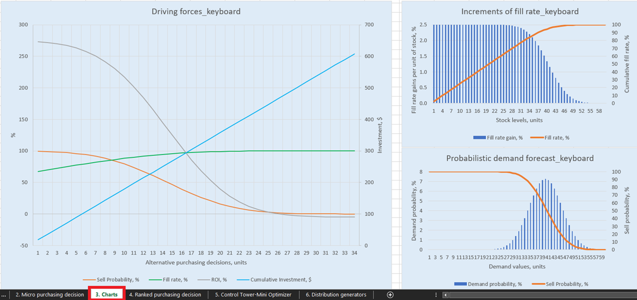
Figure 1. View of “Driving forces keyboard” in Charts, location highlighted in red.
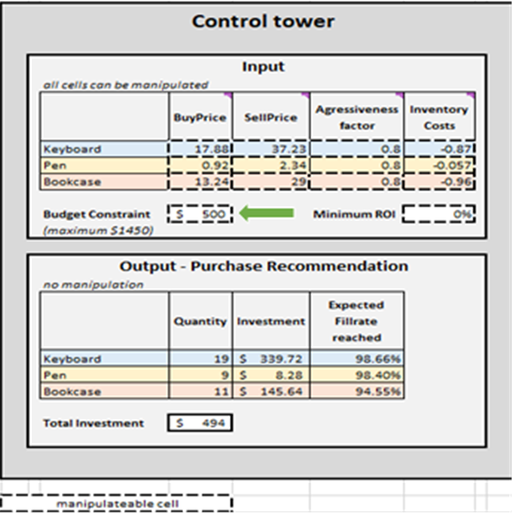
Figure 2. View of “Control Tower” located in Control Tower – Mini Optimizer (sheet 5). One can edit the “Budget Constraint” to any value between $0 and $1450 (see green arrow).
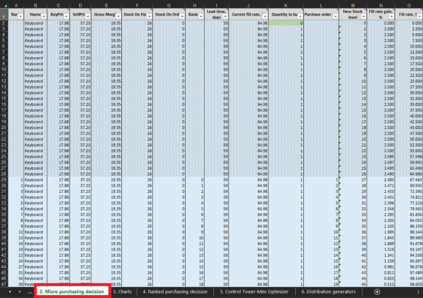
Figure 3. Where to locate Micro purchasing decisions within Excel, highlighted in red. The rows covered by conditional, dotted formatting are past data (up to and including line 28 in the above image). This information represents previous purchasing decisions. We are only concerned with everything below this conditional formatting. The same dotted formatting applies to the pen and bookcase data.
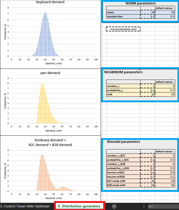
Figure 4. Where to locate Distribution generators within Excel, highlighted in red. Product control panels are highlighted in blue. The cells with dashed contours can be manipulated.
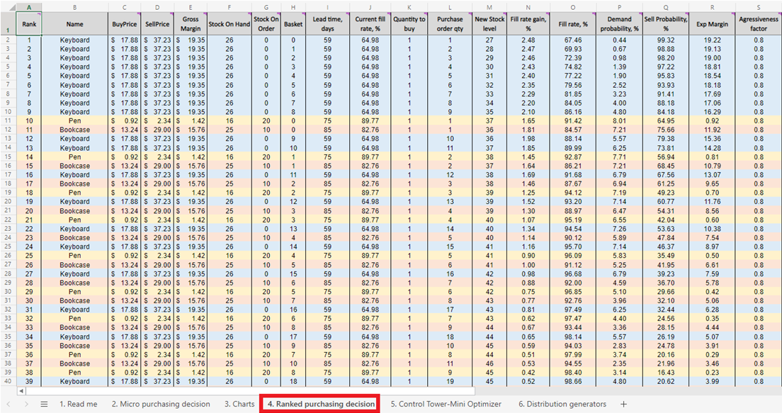
Figure 5. A prioritized inventory replenishment list of micro purchasing decisions, located in sheet 4.
2. Probabilistic Demand Forecast
In this context, a probabilistic forecast is a set of all probable future demand values and their respective probabilities. It embraces the inherent uncertainty of future demand and can be built over any time period. Like a traditional time series forecast, there is a single, most probable demand value identified (the white dots in Figure 6) and a trend line (the grey line connecting the white dots). However, a probabilistic forecast integrates uncertainty through the addition of all possible (though not equally probable) demand values. This approach can be seen in Figure 6, where different confidence intervals represent demand values with different probabilities.
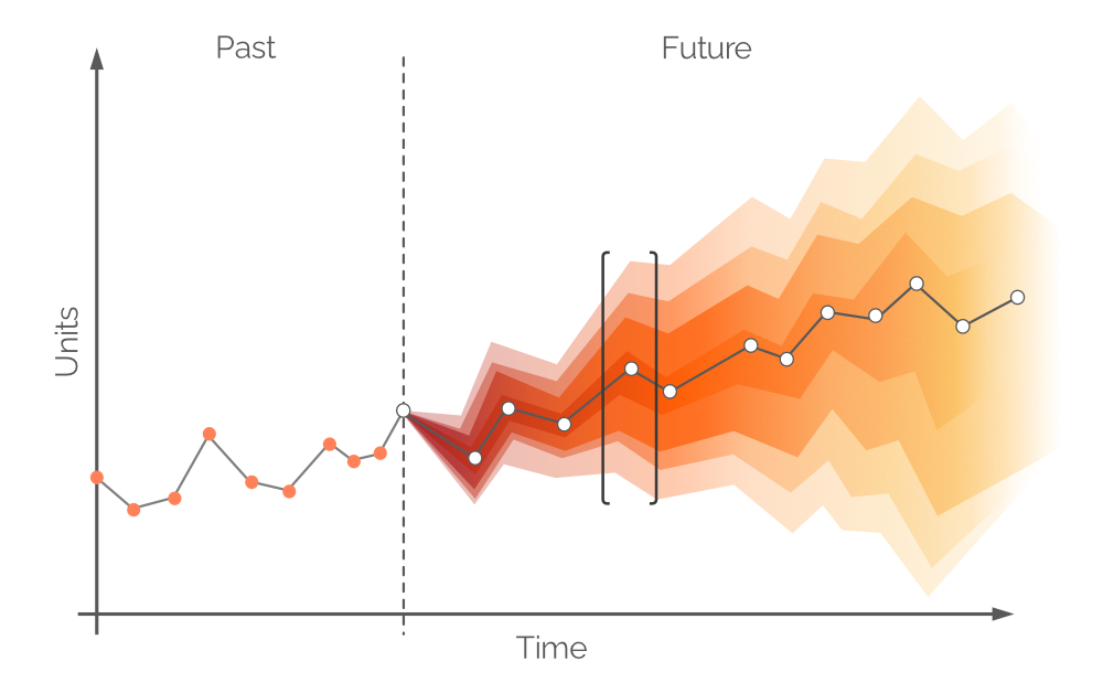
Figure 6. A probabilistic forecast (demand on y-axis; time on x-axis). The dashed vertical gray line indicates the current moment (“now”). Time is measured in days, though this could be any desired interval. The area in black brackets is discussed later.
The white dots in Figure 6 represent the most probable demand values at fixed future intervals. There is an accompanying color band that corresponds to a range of alternative future demand values - a probability distribution in color. This color fades along the vertical axis the farther one gets from the white dot, representing the greater uncertainty and lower probability. Overall, the color bands fade as time progresses (along the horizontal axis), as uncertainty intensifies with the passing of time. However, regardless of uncertainty, there is always at least one value that is the most probable, and this is represented at all times by the white dots. An example of a probability distribution for one time point is illustrated in Figure 7.
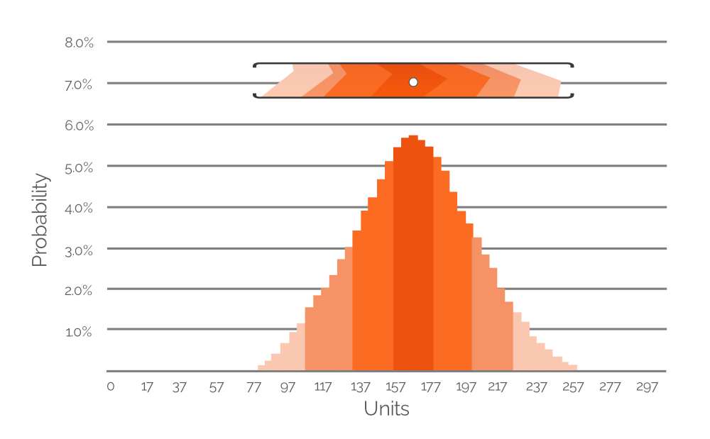
Figure 7. A histogram depicting the probability of several possible demand values (at 20-unit intervals). Y-axis is probability value; x-axis is demand in units. The histogram is a representation of the highlighted value range in Figure 6 (included here for reference purposes).
Figure 7 expresses the highlighted data from Figure 6 as a probability histogram, with explicit numerical values denoting the probability of different demand values. The color-coding is maintained for ease of comprehension (remember, fainter colours are less probable; denser colours are more probable). In this example, the most probable demand value is 167 units (+/-), which is why the white dot in the cropped value range from Figure 6 is positioned directly above the tallest bar in the histogram. However, we also assign demand probabilities to extremely low and high demand values (around 80 and 260 units, respectively, both of which are very faint orange). This demonstrates the potential data richness of a probabilistic forecast and similar histograms are included in the Excel spreadsheet - one for each of our SKUs (see Figure 4). Using these histograms (like in Figure 7 above), demand values (in units) with nonzero probabilities of occurrence can be identified and factored into the PIR.
2.1 The Construction of a Probabilistic Forecast
Though it is possible to build a real probabilistic forecast with historical data in Excel, it is arguably the least capable tool for this purpose. Overall, the specifics of building a production grade probabilistic forecast are beyond the scope of this document, hence synthetic probabilistic forecasts were selected for simplicity. The parameters of these synthetic forecasts can be manipulated in Distribution generators (see Figure 4). It is, however, recommended that one first studies the default settings before making adjustments.
In mainstream supply chain practices, demand is typically considered to be normally distributed, however this is a rarity. In real-world supply chains, most SKUs deviate from normal distribution patterns. Given this reality, we deliberately selected three different distribution patterns: normal (for keyboards), negative binomial (for pens) and bimodal (for bookcases - a mixture of two negative binomial patterns). The following provides justification for this assumption.
For example, we assume that bookcases are bought by both individuals and companies (e.g., schools), hence we use a bimodal distribution. In the default bookcase setting, there is frequent demand from individuals, with one or two units purchased per customer. This represents the first mode of the distribution (see Figure 4). Companies, however, represent less frequent demand sources but make bigger orders (bigger than individuals tend to). When this happens, their demand is added to the demand generated by individuals’ purchases, and the second mode of the distribution appears. This second mode is shifted to the right (representing high demand values), and is noticeably smaller than the first mode, reflecting the fact that it happens less frequently (Figure 4). Our model also assumes that pens are bought by individuals with infrequently high demand (students buying before school exam dates, for example). Finally, to reflect the fact that a normal distribution does occasionally occur, keyboard sales follow a normal distribution pattern.
Within Distribution generators (Figure 4), one can edit demand distributions by changing the parameters in the manipulatable cells. For example, increasing the mean for keyboards (see “NORM parameters” in Figure 4) from 40 to 50 will result in the distribution shifting 10 units to the right. As a result of this increase in mean demand, the expected ROI for all keyboard units will increase. Similarly, one can make modifications to the parameters of the negative binomial (pens) and bimodal (bookcases) distributions.
As Excel lacks the expressiveness for this kind of calculation, this demonstration limits modifications to 100 units per product. For example, setting the keyboard mean to 99 will result in almost 50% of the demand units failing to compute in the Micro purchasing decisions sheet.
2.2 Selecting a Horizon for a Probabilistic Demand Forecast
Typically, forecasts are divided into daily/weekly/monthly intervals, though these discrete periods are of limited utility and value from a replenishment perspective. Demand over the next lead time cannot be covered by purchasing decisions made today unless backorders are allowed, because any units purchased will arrive after a period equal to the lead time. Thus, demand should be covered with the store’s stock on hand and stock on order (see Figure 8), assuming the on order units arrive prior to the demand. Therefore, the probabilistic forecast is concerned with the demand between reorder points or, in other words, the demand during Reorder period 1 (see Figure 9). More distant future demand will be covered with future orders (see Reorder period 2, in Figure 9).

Figure 8. Stock on Hand (column F) and Stock on Order (column G), highlighted in red, are located in Micro purchasing decisions. Lead time, column I, is highlighted in blue.
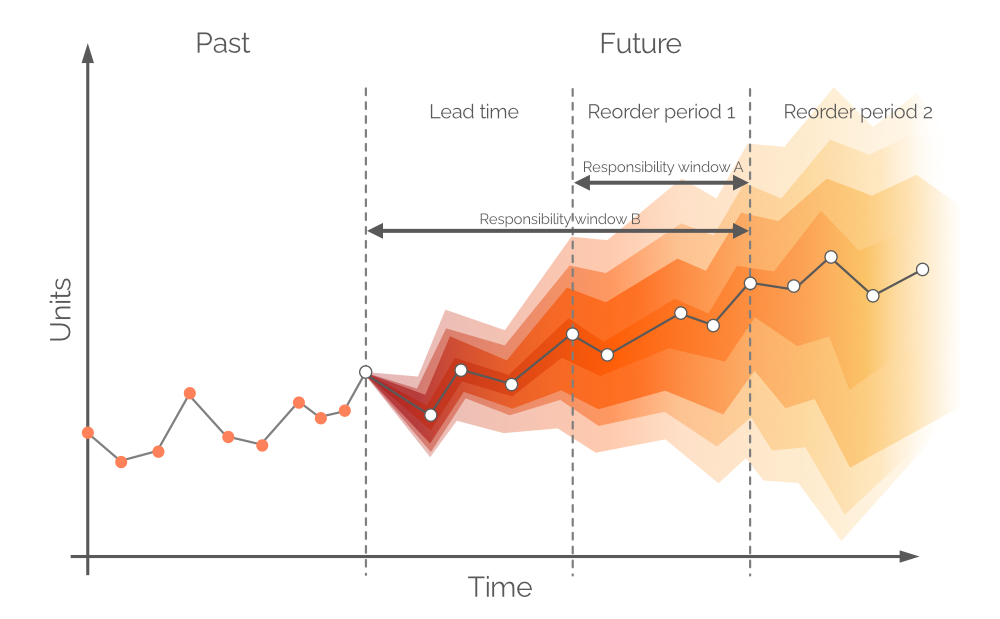
Figure 9. A visual depiction of alternative responsibility windows. Demand is on the y-axis, time on the x-axis, with the dashed vertical gray line on the left indicating the current moment (“now”, as per Figure 6). The probabilistic forecast in this document is concerned with demand over the horizon equal to Responsibility window B.
In theory, the probabilistic demand forecast should be built over the time frame equal to Reorder period 1 - this window of time is referred to as Responsibility window A (see Figure 9). In order to do this, we would need to make future projections for stock on hand and stock on order at the end of lead time. However, demand over lead time – for which we already made decisions during the previous order period – is also probabilistic, and this would result in stock levels that are probability distributions themselves3. By allowing backorders (a common practice in some verticals) a probabilistic forecast can be built over a joint period (Lead time plus Reorder period 1, as per Figure 9, aka Responsibility window B).
It can be assumed that current levels of stock on hand and stock on order will serve demand during the lead time period. If there is a stockout event, any subsequent demand will be covered with backorders. These backorders will be served by the micro purchasing decisions taken as of today. This allows us to treat stock on hand and stock on order as discrete values (instead of random ones)4.
3. Identifying Feasible Replenishment Decision Options
In a real inventory replenishment scenario, one would need to outline all feasible decision options, because there is no straightforward way to transition from a probabilistic forecast to the single best decision (purchase quantity, in this case) for every product. Instead of a single perfect choice, a probabilistic approach presents a range of possible decisions that one must consider in terms of feasibility.
Feasibility here has the pedestrian meaning that a decision is immediately actionable; it can be executed “as is” without further computations or checks. For instance, a decision is “feasible” if it is profitable and satisfies all our constraints (e.g., MOQs, EOQs, lot sizes, full container shipments, and any other constraint that may exist in our supply chain)5.
At every line of the Micro purchasing decisions sheet (Figures 3 and 10), we must consider adding one more unit of stock to our purchase order for a particular product6. Our “present” (or Day 1 of this experiment) begins at line 29, which shows the current stock level. This is calculated as a sum of Stock On Hand and Stock On Order. If we decide to add a unit to the purchase order then the overall purchase quantity will be computed in Column L as the sum of all units considered so far for purchasing (see notes in Figure 10).
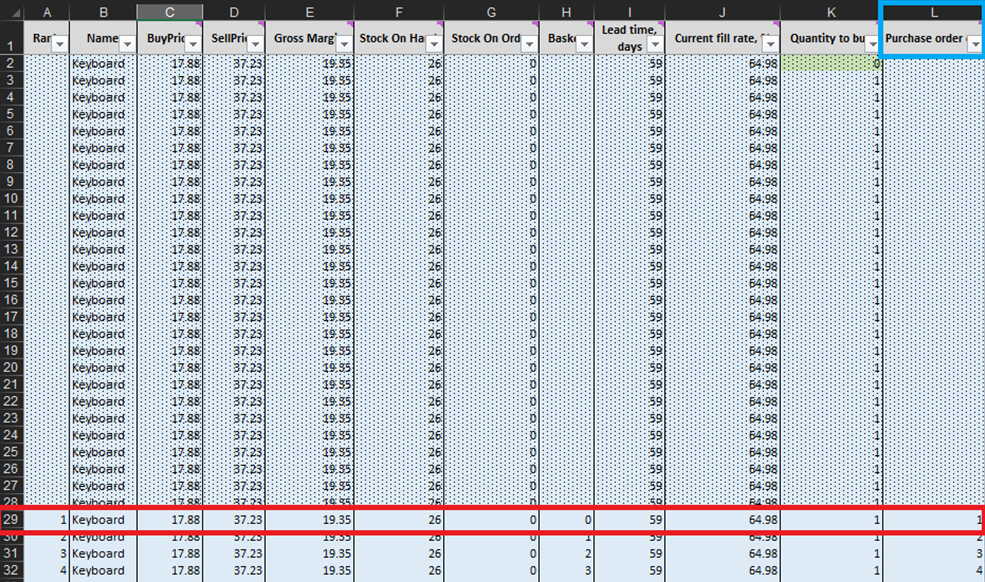
Figure 10. View from within Micro purchasing decisions sheet. Line 29, highlighted in red, is where our experiment begins (for keyboards). Purchase order column is highlighted in blue. The same principle applies to lines 140 (for orders of pens) and 240 (for orders of bookcases).
Once these feasible inventory decisions have been identified, we will calculate and rank the economic reward of every possible purchase. Note that we do not evaluate the purchase reward for units that are currently either stock on hand or stock on order (columns F and G in Figure 10). Given we already bought these units, the theoretical economic reward was determined (and ranked) at a previous date. For example, if we look at the keyboard data in Figure 10, there are currently 26 units in stock. Thus, we will start computations at line 29 and consider if we should order our first unit of additional stock (which would raise the stock levels from 26 to 27 units).
3.1 Evaluating Feasible Purchasing Decisions
In order to choose the best purchase quantity for every product, it is necessary to compute the expected monetary return at the unit level for every feasible quantity for every product (considering the uncertain future represented by the probabilistic forecast). This is an expected value concept adapted to the most granular level of inventory decision-making.
In reality, every kind of economic driver should be considered when trying to compute the expected return for every feasible decision7. For the purposes of this demonstration, here are the factors that we will consider:
- Sell price: How much we charge customers for the product.
- Carrying/Storage cost: How much it costs for us to hold the product.
- Buy price: How much it cost for us to buy the product from our supplier/wholesaler.
- Stockout cover: Covered below in detail as it is a lesser-known but nevertheless important driver8.

Figure 11. Explanatory note for Buy Price, viewable by hovering over the column header. There is a definition for each column in each sheet of the Excel document.
Stockout cover represents a financial incentive to keep a unit of a product in stock, but not with the explicit goal of selling it. This economic driver is used to model the relative importance of a product to other ones. It incentivizes avoiding a stockout event for products that might be seen as less important due to their direct margin contributions, as these products may significantly contribute to profit margins in an indirect way. As such, it is more akin to a reward driver9. Though this driver is fuzzy, it is crucial to identify all critical products (even ones that are not direct margin drivers).
3.2 Calculating Each Feasible Decision’s Score
The total economic consequence (or purchase reward) of an inventory replenishment decision is the sum of all economic drivers, including expected margin, expected inventory cost, and stockout cover (defined in detail below). Storage cost is included in these calculations as a negative driver, acting as counterforce to balance our inventory replenishment decisions.
Below is an analysis of the economic implications of the formulas in each column, using line 29 of the Micro purchasing decisions sheet as an example (see Figure 12)

Figure 12. A breakdown of the drivers per key columns, using line 29 of Micro purchasing decisions (Excel sheet 2). Certain columns were hidden for the convenience of the figure.
To compute the expected reward for each decision we need the following drivers:
Gross margin (column E) = Sell price – Buy Price.
Sell probability (column Q) = check formula in sheet10.
Not sell probability (no column) = 100% - Sell Probability
Expected margin (column R) = Gross margin * Sell Probability/100.
Aggressiveness factor (column S) = Ranges from 0 to 1. 0.8 selected for this tool.
Stockout cover (column T) = Sell price * Aggressiveness factor * Sell probability
Storage cost (column U)
Expected inventory cost (column V) = Storage cost * not sell probability11.
Using the above data, the purchase reward for every micro-level inventory decision (every unit of every product) is computed as follows:
Purchase reward (column W) = Expected margin + Stockout Cover + Expected inventory cost.
Once we have the purchase reward estimation we can compute the final score that we will later use to rank all considered decisions.
Score (column Y) = Purchase reward / Investment (column X)12.
Given stockout cover is a fuzzy driver that incorporates both direct and indirect returns, purchase reward is not a strict reflection of an inventory decision’s expected return in isolation. If one wishes to calculate this type of return, one would exclude stockout cover from this formula13.
4. Ranking Feasible Inventory Replenishment Decisions
Once we have the score for every feasible inventory purchasing decision (for every product), a list is generated and sorted in descending order (highest to lowest) in Ranked purchasing decisions (see Figure 13). Each feasible inventory decision is sorted in terms of positive ROI %. An ordinal ranking (1st, 2nd, 3rd, etc.) is also assigned to each decision (see column A in same figure).
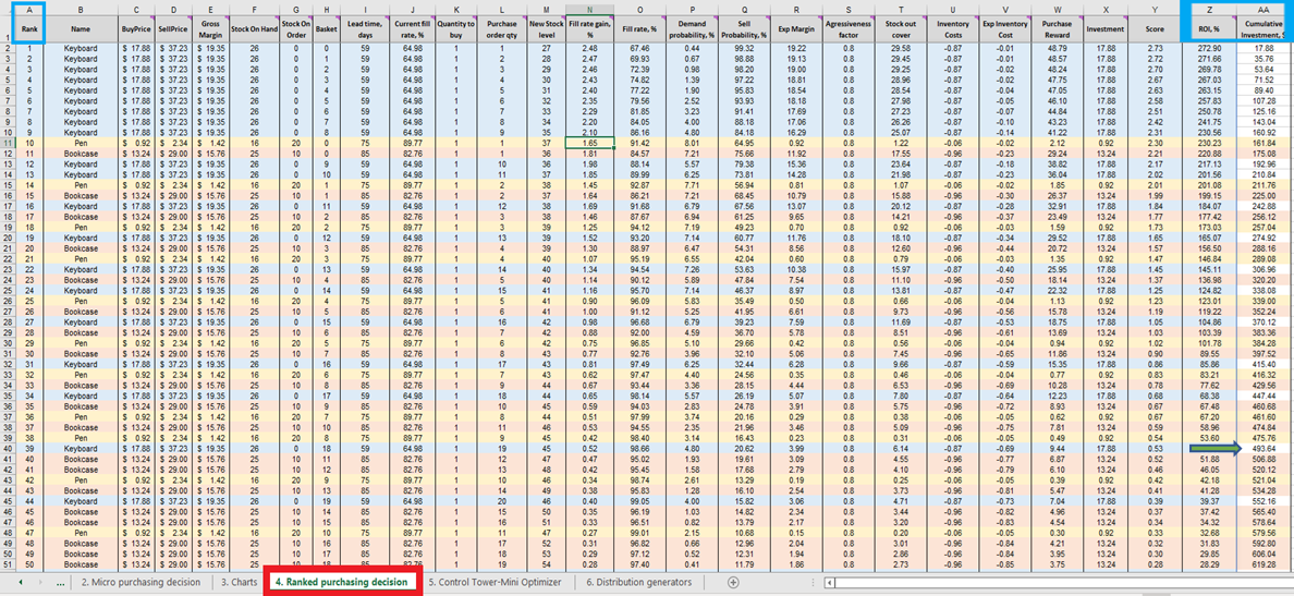
Figure 13. Ranked purchasing decisions location highlighted in red. Columns A, Z and AA are highlighted in blue. Cell 40 (the cut-off point for a $500 budget – the spreadsheet’s default) is indicated by the green arrow.
Ranked purchasing decisions features color-coded rows for each product (keyboards, pens and bookcases), used here to demonstrate how the choice to add a single extra unit of any given product interacts with every other extra unit of every other product. Each of these inventory decisions collectively influence ROI. Finally, a cumulative investment value is computed (column AA, Figure 13). This can be used to indicate where one ought to terminate purchase decisions in light of one’s budget constraints - though this is only one possible termination indicator14.
5. Determining Termination Criteria
In terms of selecting a termination point (both in Ranked purchasing decisions and in reality), criteria will vary depending on a host of variables. For example, one might have a modest budget and thus maximizing ROI is problematic given especially tight margins. Alternatively, it is possible that one has an overall target for service level and must then balance this priority with a drive to maximize profit margins.
To get even more granular, one’s termination criteria could encompass a drive for maximized ROI with varying service level targets for each product or category. Termination criteria is, thus, a strategic choice that should be made after frank reflection on a company’s overarching business goals. Prioritized inventory replenishment (PIR) is remarkably flexible in this regard; termination criteria for every purchasing cycle can be adjusted utilizing the same overall ranking procedure
For explicit visualizations of our possible inventory replenishment decisions, there are three charts and graphs for each product in the Charts dashboard (sheet 3, see Figure 14). Of particular interest is “Driving forces_product name” (Keyboard example is used in Figure 14), which shows the evolution of ROI given different purchase quantities at the unit level.
As is evident in the chart, there is a point at which increased purchase quantities will result in a negative ROI. This is because, at a certain level, there is no point in buying more units as our expected margins will be critically reduced by increased expected inventory costs.

Figure 14. View of “Driving forces_keyboard” in Charts, location highlighted in red.
Once termination criteria is determined, the prioritized inventory replenishment decisions are aggregated per SKU, which in turn updates the Quantity, Investment and Expected fillrate reached in Output-Purchase Recommendation for each SKU (see Figure 15). One can alter budget constraints ($0 to $1450), which will, in turn, update the recommended purchase list. For the sake of convenience, the control tower features two additional blocks: Base Case – hard copy and Changes to base scenario. The former is static and displays the default settings for the demonstration as designed by Lokad; the latter displays the difference between any modifications made and Lokad’s default setting.
The purchase recommendation list in Control tower represents the goal of this demonstration (see Figure 15).
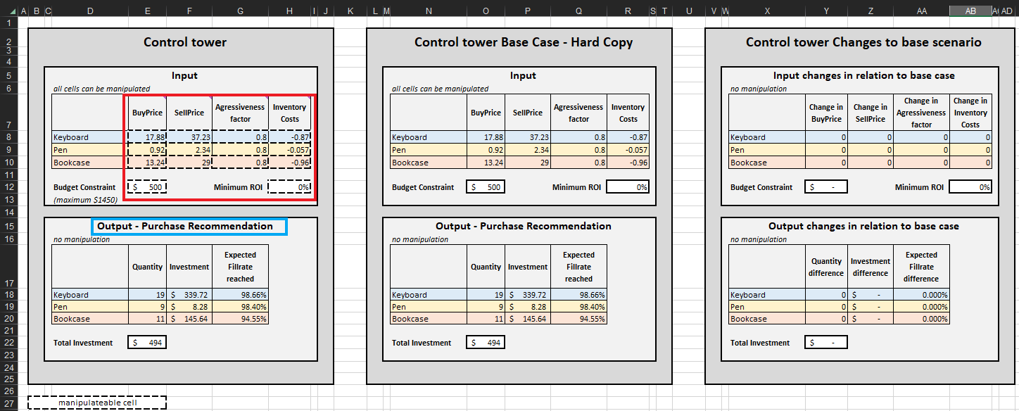
Figure 15. View of Control Tower-Mini Optimizer (sheet 5). The manipulatable cells are highlighted in red. “Purchase recommendation” is highlighted in blue and represents the goal of a prioritized inventory replenishment approach.
6. Conclusion
Traditional time series forecasts are simply incapable of capturing the level of granularity necessary to make inventory replenishment decisions that reflect future uncertainty and the full scale of one’s constraints and drivers. This is because they lack an explicit uncertainty dimension, represented by probability values for expected future outcomes. As a traditional time series is effectively blind to this type of data, a classic coping method like safety stock amounts to guesswork; not enough and one loses profitable sales with positive expected ROI; too much and one reduces one’s ROI by stocking units that (as demonstrated in the spreadsheet) have negative expected ROI.
Prioritized inventory replenishment, utilizing probabilistic forecasts, is our solution to this problem. Such an approach considers inventory replenishment choices in combination, rather than in isolation. By doing so, the expected financial reward of our inventory replenishment choices can be fully quantified and revealed. The foundation of such an approach is embracing uncertainty and leveraging probabilistic forecast inputs. In turn, one can also gain greater insight into what service levels (per SKU) yield meaningful financial rewards, rather than setting arbitrary targets.
The PIR approach demonstrated in this document was constructed using synthetic data and narrow parameters. These choices were made to adapt a common tool (Excel) to an uncommon purpose (PIR). Amongst other necessary concessions, SKUs and units were limited (to 3 and 100, respectively) to reduce processing time, as an entire catalog’s worth of data (let alone multiple stores’ data) would be too laborious to process. Further, no supply chains constraints were added. Crucially, Excel is not designed to process random variables - a key step in generating probabilistic forecasts and PIR policy. These limitations do not apply to a production grade PIR solution.
Supply chain practitioners whose businesses have outgrown Excel are welcome to email contact@lokad.com to arrange a demonstration of a production grade PIR solution.
7. Overview of the Spreadsheet
7.1 Read Me
This sheet serves as the landing page for the user. There is a link to an online tutorial (the one you are reading now).
7.2 Micro purchasing decisions
This is the second sheet and is dedicated to fine granular financial analysis of all feasible replenishment decision options. Please note that no manual data manipulation is performed here. This sheet only displays the results of computations based on inputs from the Control Tower and Distribution generators sheets.
Key features:
- Rows with conditional formatting are “past decisions” and cannot be altered. We recommend using a desktop app as Excel’s browser-based one is sometimes unreliable in terms of formatting.
- Hovering over each column header will reveal a helpful definition/note.
7.3 Charts
This is the third sheet and is dedicated to visualizing the main drivers at play in one’s inventory replenishment decisions. Please note that no manual data manipulation is performed here. This sheet is designed to help the practitioner visualize (and thus better understand) the inner-workings of the PIR process.
Key features:
- Three graphs per SKU (keyboard, pen, and bookcase).
- The “driving forces” chart visualizes the main driving forces for each decision at the unit level (for each SKU). This is why the x-axis contains only units of a SKU that are yet to be ordered.
- Two other charts (“increments of fill rate” and “probabilistic demand forecast”) contain all units of stock – stock on hand and the units that can be ordered.
7.4 Ranked purchasing decisions
This is the fourth sheet and is dedicated to listing all feasible replenishment decisions, sorted by ROI/score in descending order. This list is automatically sorted from sheet 2 data (Micro purchasing decisions). Feasible decisions are displayed in relation to each other (see “Key features” below). Please note that no manual data manipulation is performed here. Depending on changes made to the inputs in sheets 5 and 6, this list will change.
Key features:
- Feasible inventory replenishment decisions are ranked in descending order (highest to lowest) by ROI/score.
- Cumulative investment is computed for the sorted decisions (see column AA in sheet 4).
- Hovering over each column header will reveal a helpful definition/note.
7.5 Control tower-mini optimizer
This is the fifth sheet and summarizes the model assumptions (inputs) and the recommended decisions (outputs). Data in manipulatable cells can be changed to alter the model assumptions and therefore the model’s output.
Key features:
- Three blocks to assist in the demonstration: “Control tower” for manual manipulation of inputs; “Base Case – Hard copy” to display the default settings; and “Changes to base scenario” to display the difference between the updated and default settings (see sheet 5).
- A fourth block (“Model Assumptions”), located under “Control tower”, is dedicated to manipulating the initial stock assumptions (see sheet 5).
- Only data in manipulatable cells can be changed.
7.6 Distribution generators
This is the sixth sheet and is dedicated to the generation of probabilistic demand forecasts. Parameters in manipulatable cells can be changed, which will result in the distributions updating and displaying new probability demand values.
Key features:
- One distribution graph per SKU.
- Each SKU has a different distribution pattern (reasoning explained in section 2.1).
- There is a table to the left of the series of distribution graphs, dedicated to manipulating parameters of the distributions.
- Only parameters in manipulatable cells can be changed.
- Hovering over relevant column headers (in the table) will reveal a helpful definition/note.
Notes
-
Consider milk and chocolate. The former is a low margin product, yet it is considered a staple, while the latter is discretionary with higher profit margins. People tend to buy staples and discretionary products together, but the penalty for not having milk is different than for chocolate. A customer may swap one discretionary product (biscuits) for another (chocolate) in the case of a stockout, but if they cannot buy a staple (milk), they may leave the store altogether. This is why the stockout cover would be greater for milk than chocolate, regardless of gross profit margin. From our perspective, stockout cover is a reward rather than a penalty, as it is intended to enable greater sales. ↩︎
-
Three products are enough to illustrate the concept but also keep the document concise and digestible. ↩︎
-
Stock levels become probabilistic as we subtract probabilistic demand from discrete values of stock (discrete value minus probability distribution yields another probability distribution). All of this would make it too complicated to explain things through Excel, as it is not suited to performing computations with random variables (think ‘demand probability distributions’). ↩︎
-
These concessions are necessary to demonstrate the overall principle of a probabilistic approach. In reality, backorders are not always used and lead times are probabilistic and subject to change. ↩︎
-
For the sake of simplicity, we did not apply any supply chain constraints. ↩︎
-
As mentioned previously, we do not need to edit any data in Micro purchasing decisions. All data manipulation is conducted via sheets 5 and 6. ↩︎
-
In this Excel sheet, economic drives are expressed in dollars, though currency is irrelevant. ↩︎
-
The list of economic drivers above is not comprehensive and real inventory replenishment (and supply chain) scenarios will almost certainly feature more. This is especially true when dealing with the production of goods and perishability constraints. ↩︎
-
This driver is fuzzier in a B2C context than a B2B one. For the latter, there are often explicit penalties associated with stockout events, such as contractual penalties; for the former, it is difficult to financially quantify the negative impact of a stockout event. Generally, it will be high for products that inflict a disproportionately negative toll on a business’ attractiveness (regardless of the SKU’s direct margin contribution). Milk, as covered earlier, is not a margin driver for supermarkets, but its strategic placement (usually at the back of the supermarket) prompts customers to walk through aisle after aisle of other products (almost all of which have higher margins). If a supermarket experiences a stockout event with this staple product (one that people tend to buy very regularly and in baskets), this may drive customers to leave the supermarket, shop elsewhere, and possibly not return (if these stockout events are regular). ↩︎
-
Sell probability is derived from probability distributions generated in Distribution generators (sheet 6). ↩︎
-
The ongoing cost for failing to sell and thus having to store an unsold unit of a SKU. ↩︎
-
The investment is, in this scenario, the same as the buy price, but only because our purchasing decisions are not constrained by MOQs or lot multipliers. ↩︎
-
The easiest way of doing this is to set aggressiveness factor (column S in Figure 12) to zero, which a business could do if they decided that a stockout event has no negative impacts. Some free advice: it definitely does. ↩︎
-
For example, our default budget is $500, so we would terminate our purchasing decisions at cell 40 (see Figure 13), as cell 41 has a value of $506.88 and is beyond our budget. We would then aggregate numbers per product, which would constitute our purchase list (see Output – Purchase recommendation in Control Tower, as per Figure 2). As previously mentioned, one can edit the pre-set $500 budget (see Figure 2 for directions) to any value between $0 and $1450. This will demonstrate how the purchase list changes with different budget constraints. Regardless of financial limitations, Ranked purchase decisions will identify the best possible combination of inventory decisions, from an ROI perspective, for all rows between rank 1 and the termination point. ↩︎